Lecture 8 Estimating Pre-exponential Factors

8.1 From Molecular Freedom to Reaction Rates

In Lecture 7, we examined how molecular degrees of freedom change when forming the activated complex, and how these changes determine the entropy of activation, $\Delta S^\ddagger$. We saw that forming the activated complex typically transforms high-entropy translational and rotational degrees of freedom into more constrained rotational and vibrational modes. Let us now develop this molecular-level picture into a quantitative framework for predicting reaction rates.

To understand how molecular motion leads to reaction, we must look more carefully at what the reaction coordinate means. Consider a simple atom-transfer reaction A + BC → AB + C. For simplicity, we assume the reaction proceeds through a collinear arrangement of the three atoms. We can then describe the molecular geometry using two key distances: the A–B distance ($r_\mathrm{AB}$) and the B–C distance ($r_\mathrm{BC}$).

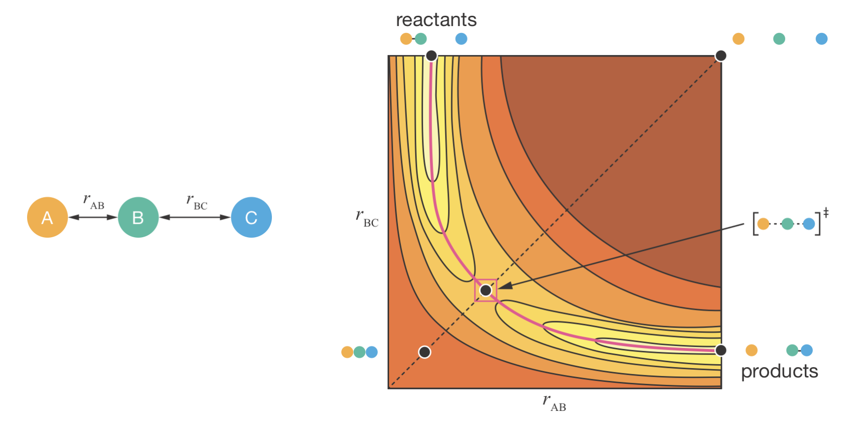
$The reaction coordinate for a bimolecular exchange reaction A + BC → AB + C. Left: The two key bond distances that define the reaction coordinate. Right: The potential energy surface as a function of $r_{\mathrm{AB}}$ and $r_{\mathrm{BC}}$. Five key configurations are marked on the surface: reactants (top left), products (bottom right), transition state (centre saddle point), and two high-energy configurations at the remaining corners. The reaction coordinate (pink line) follows the minimum energy pathway connecting reactants, transition state, and products.$

Figure 8.1: The reaction coordinate for a bimolecular exchange reaction A + BC → AB + C. Left: The two key bond distances that define the reaction coordinate. Right: The potential energy surface as a function of $r_{\mathrm{AB}}$ and $r_{\mathrm{BC}}$. Five key configurations are marked on the surface: reactants (top left), products (bottom right), transition state (centre saddle point), and two high-energy configurations at the remaining corners. The reaction coordinate (pink line) follows the minimum energy pathway connecting reactants, transition state, and products.

Figure 8.1 shows the potential energy surface for this reaction. At the reactants (top left), $r_\mathrm{AB}$ is small (corresponding to a strong A–B bond) whilst $r_\mathrm{BC}$ is large (C is far from the AB molecule). Conversely, at the products (bottom right), $r_\mathrm{AB}$ is large (A has separated) whilst $r_\mathrm{BC}$ is small (a strong B–C bond has formed).

Between these two stable configurations, the system must pass through the transition state—the dividing surface that separates reactant-like from product-like configurations. The lowest-energy point on this dividing surface is the saddle point (centre of the surface), where both $r_\mathrm{AB}$ and $r_\mathrm{BC}$ have intermediate values. The molecular arrangement at this saddle point, with the AB bond partially broken and the BC bond partially formed, is the activated complex.

The remaining two corners represent high-energy configurations the system avoids: all atoms separated (top-right) or impossibly compressed together (bottom-left). The reaction coordinate (pink line) follows the minimum-energy pathway that connects reactants to products through the saddle point, avoiding these unfavourable regions.

8.2 The Rate of Barrier Crossing

To describe how fast activated complexes convert to products ($k^\ddagger$), we need to think about what happens at the transition state. Consider again our simple atom-transfer reaction A + BC → AB + C, shown in Figure 8.2.

$Motion across the transition state for the reaction A + BC $\to$ AB + C. Left: The molecular geometries along the reaction coordinate, showing reactants (top), the transition state activated complex [A⋯B⋯C]$^\ddagger$ with both bonds partially formed (centre), and products (bottom). Right: A zoomed-in view of the saddle point region from Figure \@ref(fig:reaction-coordinate), showing the transition state on the potential energy surface. Motion along the reaction coordinate (pink line) corresponds to vibration-like motion through the transition state, with frequency $\nu^\ddagger = k_\mathrm{B}T/h$.$

Figure 8.2: Motion across the transition state for the reaction A + BC $\to$ AB + C. Left: The molecular geometries along the reaction coordinate, showing reactants (top), the transition state activated complex [A⋯B⋯C]$^\ddagger$ with both bonds partially formed (centre), and products (bottom). Right: A zoomed-in view of the saddle point region from Figure 8.1, showing the transition state on the potential energy surface. Motion along the reaction coordinate (pink line) corresponds to vibration-like motion through the transition state, with frequency $\nu^\ddagger = k_\mathrm{B}T/h$.

At the transition state (centre of the left panel), we have an activated complex [A⋯B⋯C]$^\ddagger$ where both bonds are partially formed. What happens if we move a small distance along the reaction coordinate? The right panel shows a zoomed-in view of the saddle point region from Figure 8.1. Motion along the pink line through this saddle point corresponds to changes in both bond distances simultaneously: moving towards reactants, $r_\mathrm{AB}$ decreases and $r_\mathrm{BC}$ increases; moving towards products, $r_\mathrm{AB}$ increases and $r_\mathrm{BC}$ decreases.

This motion through the transition state resembles an asymmetric stretch of the activated complex—a vibration-like mode where the system oscillates along the reaction coordinate. By modelling this as a loose molecular vibration, we can derive the expression:

\[k^\ddagger = \frac{k_\mathrm{B}T}{h}\]

where $k_\mathrm{B}$ is Boltzmann’s constant, $h$ is Planck’s constant, and $T$ is temperature.⁵ Because this expression accounts for motion along the reaction coordinate, we must take care when counting vibrational modes in the activated complex: we always count one fewer vibrational mode than the molecular geometry would normally possess ($3N-6$ for a linear complex instead of $3N-5$, or $3N-7$ for a non-linear complex instead of $3N-6$), as the reaction coordinate “vibration” is already included in the $k^\ddagger$ term.

8.3 Mathematical Development

Having established how to treat motion across the transition state, we can now develop the complete mathematical framework for estimating pre-exponential factors. We will combine our expression for $k^\ddagger$ with the entropy of activation to derive a working equation that connects molecular properties to reaction rates.

The complete transition state theory rate equation can now be written as:

\[\nu = \frac{k^{\ddagger}}{c^\circ}\mathrm{e}^{\Delta S^{\ddagger}/R}\mathrm{e}^{-\Delta H^{\ddagger}/RT}[\mathrm{A}][\mathrm{B}]\]

Comparison with the Arrhenius equation:

\[\nu = A\mathrm{e}^{-E_\mathrm{a}/RT}[\mathrm{A}][\mathrm{B}]\]

reveals that the pre-exponential factor corresponds to:

\[A \approx \frac{k^{\ddagger}}{c^\circ}\mathrm{e}^{\Delta S^{\ddagger}/R}\]

By separating the entropy of activation into contributions from different types of molecular motion, we arrive at the complete transition state theory expression:

\[A = \frac{k_\mathrm{B}T}{hc^\circ}\mathrm{e}^{\Delta S^{\ddagger}_\mathrm{trans}/R}\mathrm{e}^{\Delta S^{\ddagger}_\mathrm{rot}/R}\mathrm{e}^{\Delta S^{\ddagger,(n-1)}_\mathrm{vib}/R}\]

where the superscript $(n-1)$ on the vibrational entropy term indicates that we consider one fewer vibrational mode than might be expected, because motion along the reaction coordinate is already accounted for in the frequency prefactor $\frac{k_\mathrm{B}T}{h}$. This expression is particularly powerful because it allows us to make quantitative predictions of the Arrhenius pre-exponential factor if we can evaluate (or estimate) the changes in translational, rotational, and vibrational entropy when forming the activated complex. For gas-phase reactions, these contributions can be estimated using characteristic values:

Translational motion: $S^{\ddagger}_\mathrm{trans} \approx 195~\mathrm{J}~\mathrm{K}^{-1}~\mathrm{mol}^{-1}$
Rotational modes: $S^{\ddagger}_\mathrm{rot} \approx 20~\mathrm{J}~\mathrm{K}^{-1}~\mathrm{mol}^{-1}$
Vibrational modes: $S^{\ddagger}_\mathrm{vib} \approx 5~\mathrm{J}~\mathrm{K}^{-1}~\mathrm{mol}^{-1}$

8.4 Analysis of Molecular Systems

8.4.1 Atomic Reactions

The simplest case to analyse is a reaction between two atoms, A + B. Initially, the system possesses:

Three translational degrees of freedom for atom A
Three translational degrees of freedom for atom B
No rotational or vibrational modes

When these atoms combine to form the activated complex [A⋯B]$^\ddagger$, this transforms into:

Three translational degrees of freedom (describing motion of the complex as a whole)
Two rotational degrees of freedom (the complex can rotate about two axes)
One vibrational mode (3N−5 = 1 for the linear diatomic complex)

From these changes in molecular freedom, we can calculate the entropy changes systematically. For translational motion, we lose three degrees of freedom when forming the complex, giving:

\[\Delta S^\ddagger_\mathrm{trans} = -3 \times 195 = -585~\mathrm{J}~\mathrm{K}^{-1}~\mathrm{mol}^{-1}\]

The activated complex gains two rotational degrees of freedom:

\[\Delta S^\ddagger_\mathrm{rot} = +2 \times 20 = +40~\mathrm{J}~\mathrm{K}^{-1}~\mathrm{mol}^{-1}\]

The activated complex has one vibrational mode, but we use N−1 = 0 modes in our entropy calculation since the reaction coordinate vibration is included in $k^\ddagger$. Thus:

\[\Delta S^\ddagger_\mathrm{vib} = 0 \times 5 = 0~\mathrm{J}~\mathrm{K}^{-1}~\mathrm{mol}^{-1}\]

With these entropy changes calculated, we can now determine the pre-exponential factor:

\[A = 10^{13} \times \mathrm{e}^{-3 \times 195/8.314} \times \mathrm{e}^{2 \times 20/8.314} \times \mathrm{e}^{0 \times 5/8.314} \times (N_\mathrm{A} \times 10^3)~\mathrm{dm^3~mol^{-1}~s^{-1}}\]

\[= 2 \times 10^{11}~\mathrm{dm^3~mol^{-1}~s^{-1}}\]

The factor of $N_\mathrm{A}$ (Avogadro’s number) converts from a per-molecule basis to a per-mole basis, since our rate constant needs to work with concentrations in mol dm$^{-3}$. The factor of $10^3$ converts volumes from m$^3$ to dm$^3$, ensuring our final rate constant has the correct units of dm$^3$ mol$^{-1}$ s$^{-1}$.

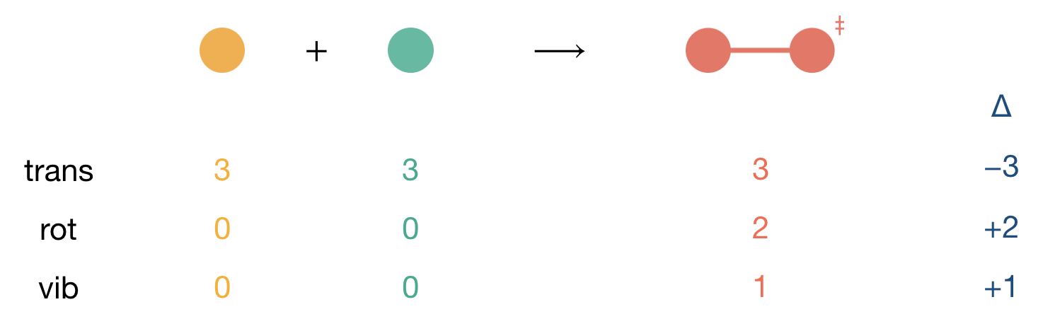
Systematic accounting of degrees of freedom changes for the reaction between two atoms. The table format provides a template for organizing similar analyses: count initial degrees of freedom for each reactant, count final degrees of freedom in the activated complex, then calculate the change (Δ) for each type of motion.

Figure 8.3: Systematic accounting of degrees of freedom changes for the reaction between two atoms. The table format provides a template for organizing similar analyses: count initial degrees of freedom for each reactant, count final degrees of freedom in the activated complex, then calculate the change (Δ) for each type of motion.

8.4.2 Polyatomic Systems

For a reaction between a diatomic molecule and a four-atom molecule, we must account for additional molecular freedom in both reactants and the activated complex. Let us examine the initial degrees of freedom systematically.

For the diatomic molecule (N = 2), being linear, we have:

Three translational modes (motion through space)
Two rotational modes (rotation about axes perpendicular to the bond)
One vibrational mode (3N − 5 = 1 for a linear molecule)

The four-atom molecule (N = 4), being non-linear, possesses:

Three translational modes
Three rotational modes
Six vibrational modes (3N − 6 = 6 for a non-linear molecule)

When these molecules combine, they form a six-atom activated complex (N = 6) with:

Three translational modes
Three rotational modes (non-linear complex)
Twelve vibrational modes (3N − 6 = 12 for the non-linear six-atom complex)

From these molecular properties, we can determine the entropy changes systematically.

For translational motion:

Initially: six independent translational modes (three per molecule)
Finally: three translational modes in the complex
Net change: $\Delta$n_trans = −3

\[\Delta S^\ddagger_\mathrm{trans} = -3 \times 195 = -585~\mathrm{J}~\mathrm{K}^{-1}~\mathrm{mol}^{-1}\]

For rotational motion:

Initially: five rotational modes (two from diatomic + three from four-atom molecule)
Finally: three rotational modes in the complex
Net change: $\Delta$n_rot = −2

\[\Delta S^\ddagger_\mathrm{rot} = -2 \times 20 = -40~\mathrm{J}~\mathrm{K}^{-1}~\mathrm{mol}^{-1}\]

For vibrational motion:

Initially: seven vibrational modes (one from diatomic + six from four-atom molecule)
Finally: twelve vibrational modes in the complex
Net change: Δn_vib = 12 − 7 = +5

However, we must use n−1 modes in our entropy calculation to avoid double-counting motion along the reaction coordinate. Using eleven modes for the complex rather than twelve, the entropy change becomes:

\[\Delta S^\ddagger_\mathrm{vib} = (11 - 7) \times 5 = +4 \times 5 = +20~\mathrm{J}~\mathrm{K}^{-1}~\mathrm{mol}^{-1}\]

With these entropy changes determined, we can calculate the pre-exponential factor:

\[A = 10^{13} \times \mathrm{e}^{-3 \times 195/8.314} \times \mathrm{e}^{-2 \times 20/8.314} \times \mathrm{e}^{4 \times 5/8.314} \times (N_\mathrm{A} \times 10^3)~\mathrm{dm^3~mol^{-1}~s^{-1}}\]

\[= 1 \times 10^8~\mathrm{dm^3~mol^{-1}~s^{-1}}\]

As in our atomic example, the factor of N_A converts to a per-mole basis, while the factor of 10³ handles the conversion from m³ to dm³ units.

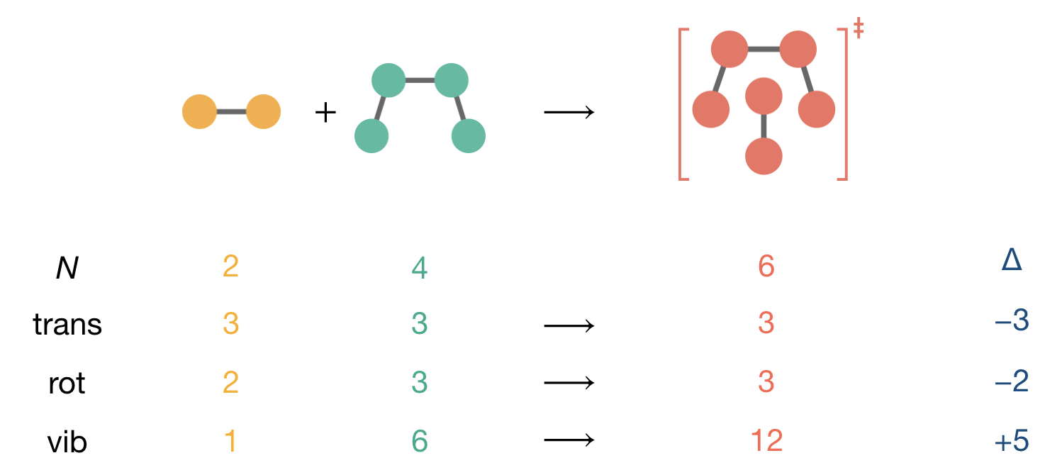
$Degree of freedom accounting for a reaction between a diatomic molecule (N = 2) and a four-atom molecule (N = 4) forming a six-atom activated complex (N = 6). The activated complex has 12 vibrational modes (3N−6 for a non-linear molecule), but when calculating the pre-exponential factor, we use only 11 modes in the entropy expression because one vibrational mode—motion along the reaction coordinate—is already included in the $k^\ddagger$ term.$

Figure 8.4: Degree of freedom accounting for a reaction between a diatomic molecule (N = 2) and a four-atom molecule (N = 4) forming a six-atom activated complex (N = 6). The activated complex has 12 vibrational modes (3N−6 for a non-linear molecule), but when calculating the pre-exponential factor, we use only 11 modes in the entropy expression because one vibrational mode—motion along the reaction coordinate—is already included in the $k^\ddagger$ term.

This more complex example reveals a key feature of molecular reactions: as molecular complexity increases, we typically observe larger decreases in molecular freedom when forming the activated complex. This systematically leads to more negative values of $\Delta S^\ddagger$ and correspondingly smaller pre-exponential factors.

8.5 Applications and Predictive Power

We now have a complete quantitative theory for predicting pre-exponential factors from molecular structure. But how do the predictions from this theory compare to experimental data?

Figure 8.5 compares our estimates with experimental values for three representative reactions spanning a wide range of molecular complexity. Our estimation method correctly predicts both the magnitude and ordering of these pre-exponential factors: the estimated values of 4 × 10⁹, 1 × 10⁸, and 2 × 10⁷ dm³ mol⁻¹ s^-1 agree with experimental measurements within an order of magnitude.

$Comparison of experimental and estimated pre-exponential factors for representative bimolecular reactions. The systematic decrease in pre-exponential factors reflects increasing molecular complexity and greater loss of molecular freedom when forming the activated complex. The estimated entropy changes ($\Delta S^\ddagger_\mathrm{rot+vib}$) become increasingly negative, leading to correspondingly smaller pre-exponential factors. Our simple estimation method successfully predicts both the magnitude and ordering of experimental values, with agreement typically within an order of magnitude.$

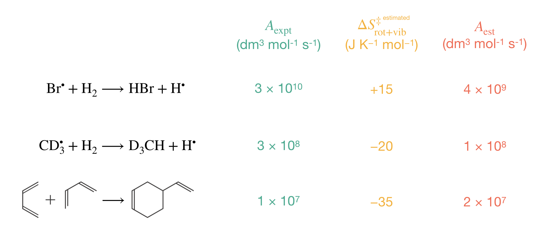
Figure 8.5: Comparison of experimental and estimated pre-exponential factors for representative bimolecular reactions. The systematic decrease in pre-exponential factors reflects increasing molecular complexity and greater loss of molecular freedom when forming the activated complex. The estimated entropy changes ($\Delta S^\ddagger_\mathrm{rot+vib}$) become increasingly negative, leading to correspondingly smaller pre-exponential factors. Our simple estimation method successfully predicts both the magnitude and ordering of experimental values, with agreement typically within an order of magnitude.

The systematic decrease in pre-exponential factors across these reactions reflects three key features:

Increasing molecular complexity in the reactants
Greater loss of molecular freedom in forming the activated complex
Increasingly negative values of $\Delta S^\ddagger_\mathrm{rot+vib}$: +15, −20, and −35 J K⁻¹ mol⁻¹ respectively

8.6 Connection to Collision Theory

This molecular freedom framework finally provides a quantitative explanation for an observation we made in Lecture 5: collision theory’s empirical steric factor $P$ is systematically less than unity for reactions between complex molecules, and decreases as molecular complexity increases.

We can now understand why. The steric factor $P$ in collision theory appears as an empirical correction to account for the requirement that molecules must collide with appropriate orientation and alignment. From our transition state theory perspective, these geometric constraints manifest as losses of molecular freedom when forming the activated complex. Reactions between more complex molecules lose more translational and rotational freedom, leading to increasingly negative values of $\Delta S^{\ddagger}$ and correspondingly smaller pre-exponential factors.

The systematic trends in Figure 8.5 demonstrate this principle directly: as we move from simple to more complex reactions, the pre-exponential factors decrease by over three orders of magnitude. Collision theory’s “steric hindrance” is thus given a quantitative thermodynamic foundation: geometrically constrained transition states, which require significant loss of molecular freedom, are thermodynamically less favourable than less constrained transition states, leading to smaller pre-exponential factors.

8.7 Limitations in Pre-exponential Factor Estimation

While our molecular freedom approach successfully predicts systematic trends in reaction rates, several important approximations underpin these calculations. Understanding these limitations helps us recognise both the power and constraints of our theoretical framework.

8.7.1 Statistical Entropy Approximations

Our calculations employ characteristic entropy values for different types of molecular motion:

Translational motion: 195 J K⁻¹ mol⁻¹
Rotational modes: 20 J K⁻¹ mol⁻¹
Vibrational modes: 5 J K⁻¹ mol⁻¹

These values represent statistical averages derived from typical molecular behaviour. For more precise predictions, we require detailed quantum mechanical calculations of molecular energy levels, which can determine specific values for $S^\ddagger_\mathrm{dof}$ based on the actual energy spacing between quantum states. While such calculations provide greater accuracy, our simpler approach using characteristic values remains valuable for understanding trends in reactivity.

8.7.2 Effects of Molecular Symmetry

Molecular symmetry introduces additional complexity beyond simple counting of degrees of freedom. Consider these parallel reactions:

\[\mathrm{CH}_4 + \mathrm{Br}^\bullet \longrightarrow \mathrm{HBr} + \mathrm{CH}_3^\bullet\] \[\mathrm{CD}_3\mathrm{H} + \mathrm{Br}^\bullet \longrightarrow \mathrm{HBr} + \mathrm{CD}_3^\bullet\]

Our previous analysis, based purely on counting molecular degrees of freedom, predicts identical pre-exponential factors for both reactions. However, experimental measurements reveal that the CH₄ reaction proceeds approximately four times faster than the CD₃H reaction.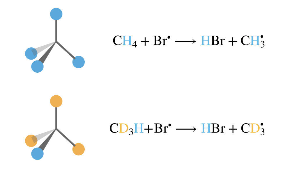

Molecular symmetry affects pre-exponential factors through configurational entropy. Top: In CH$_4$, all four hydrogen atoms (blue) are equivalent, so the bromine radical can abstract any hydrogen to form the same product, giving a statistical factor of $l = 4$. Bottom: In CD$_3$H, only one hydrogen (blue) is available for abstraction whilst the three deuterium atoms (orange) are not, giving $l = 1$. This symmetry difference results in the CH$_4$ reaction being approximately four times faster than the CD$_3$H reaction, even though simple degree-of-freedom counting predicts identical rates.

Figure 8.6: Molecular symmetry affects pre-exponential factors through configurational entropy. Top: In CH$_4$, all four hydrogen atoms (blue) are equivalent, so the bromine radical can abstract any hydrogen to form the same product, giving a statistical factor of $l = 4$. Bottom: In CD$_3$H, only one hydrogen (blue) is available for abstraction whilst the three deuterium atoms (orange) are not, giving $l = 1$. This symmetry difference results in the CH$_4$ reaction being approximately four times faster than the CD$_3$H reaction, even though simple degree-of-freedom counting predicts identical rates.

This difference arises from molecular symmetry. In CH₄, all four hydrogen atoms are equivalent—the bromine radical can abstract any hydrogen to form the same product. In CD₃H, only one hydrogen is available for abstraction.

To understand the statistical factor more deeply, consider what happens if we artificially label the four hydrogen atoms in CH₄ as shown in Figure 8.7.

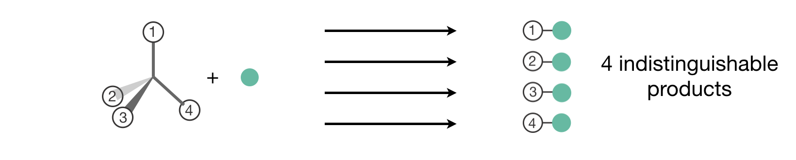
Understanding the statistical factor for CH$_4$ through artificial labeling. When we label the four equivalent hydrogen atoms (1–4), we see that reaction at each site produces a distinct labeled product. Since the hydrogens are actually indistinguishable, these represent four equivalent pathways to the same physical product, giving a statistical factor of $l = 4$.

Figure 8.7: Understanding the statistical factor for CH$_4$ through artificial labeling. When we label the four equivalent hydrogen atoms (1–4), we see that reaction at each site produces a distinct labeled product. Since the hydrogens are actually indistinguishable, these represent four equivalent pathways to the same physical product, giving a statistical factor of $l = 4$.

What we consider a single reaction is in fact four different reaction pathways—each pathway corresponds to the bromine radical extracting a different labelled hydrogen, which then gives a different labeled product. Since the hydrogen atoms in methane are actually indistinguishable, these four products, and the four reaction pathways that form them, are physically indistinguishable—all four produce the same products, CH₃• + HBr. We account for this by introducing a statistical factor, $l$, representing the number of equivalent pathways:⁶

\[A = l\frac{k_\mathrm{B}T}{hc^\circ}\mathrm{e}^{\Delta S^\ddagger/R}\]

For our example reactions:

CH₄ reaction: $l = 4$ (four equivalent hydrogens)
CD₃H reaction: $l = 1$ (single abstractable hydrogen)

The rate constant ratio becomes:

\[\frac{k_\mathrm{CH_4}}{k_\mathrm{CD_3H}} = \frac{4}{1} = 4\]

explaining the observed fourfold difference in reaction rates.

8.7.3 Internal Molecular Motion

The treatment of internal molecular motions reveals additional subtlety in our theoretical framework. Consider the ethane molecule (C₂H₆), which exhibits two distinct types of motion around its C–C bond:

C–C stretching vibration:
- Involves direct compression and extension of the C–C bond
- Requires significant energy
- Shows widely spaced quantum energy levels
- Makes small contributions to vibrational entropy
C–C torsional motion:
- Involves rotation of CH₃ groups about the C–C axis
- Requires much less energy
- Shows more closely spaced energy levels
- Makes larger contributions to entropy

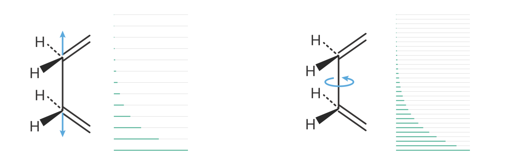
Comparison of energy level spacings for different types of molecular motion in ethane-like molecules. Left: A normal C–C stretching vibration involves compression and extension of the bond, requiring significant energy. The resulting widely spaced quantum energy levels (gray) mean only a few low-lying states (green) are thermally accessible at room temperature, giving low entropy. Right: Internal rotation of CH$_3$ groups about the C–C axis requires much less energy. The resulting closely spaced energy levels mean many states are thermally accessible, giving substantially higher entropy than a normal vibration.

Figure 8.8: Comparison of energy level spacings for different types of molecular motion in ethane-like molecules. Left: A normal C–C stretching vibration involves compression and extension of the bond, requiring significant energy. The resulting widely spaced quantum energy levels (gray) mean only a few low-lying states (green) are thermally accessible at room temperature, giving low entropy. Right: Internal rotation of CH$_3$ groups about the C–C axis requires much less energy. The resulting closely spaced energy levels mean many states are thermally accessible, giving substantially higher entropy than a normal vibration.

Figure 8.8 illustrates why internal rotation contributes more entropy than normal vibrations: the closely spaced energy levels mean many more states are thermally accessible. When molecules with internal rotations form activated complexes, two contrasting scenarios can arise:

Restricted internal rotation:
- Occurs when the transition state requires specific molecular alignment
- Reduces freedom of internal motion
- Produces more negative $\Delta S^\ddagger$ values
- Leads to lower pre-exponential factors than predicted by simple counting
Enhanced internal rotation:
- Occurs when transition state formation weakens bonds that hinder rotation
- Increases freedom of internal motion
- Produces less negative (or positive) $\Delta S^\ddagger$ values
- Leads to higher pre-exponential factors than predicted

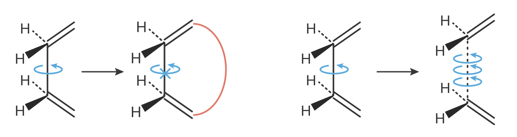
$The effect of transition state formation on internal rotation determines the sign of entropy contributions. Left: When the transition state requires specific molecular alignment or constrains rotation (indicated by the red barrier), internal rotational freedom is reduced. This produces additional negative contributions to $\Delta S^\ddagger$, leading to lower pre-exponential factors than predicted by simple degree-of-freedom counting. Right: When transition state formation weakens a bond, internal rotation becomes freer. The enhanced rotational freedom produces positive contributions to $\Delta S^\ddagger$, leading to higher pre-exponential factors.$

Figure 8.9: The effect of transition state formation on internal rotation determines the sign of entropy contributions. Left: When the transition state requires specific molecular alignment or constrains rotation (indicated by the red barrier), internal rotational freedom is reduced. This produces additional negative contributions to $\Delta S^\ddagger$, leading to lower pre-exponential factors than predicted by simple degree-of-freedom counting. Right: When transition state formation weakens a bond, internal rotation becomes freer. The enhanced rotational freedom produces positive contributions to $\Delta S^\ddagger$, leading to higher pre-exponential factors.

This effect is not limited to simple molecules. Diels-Alder cycloadditions provide a clear example: our predictions typically overestimate the experimental pre-exponential factors for these reactions. This occurs because the transition state requires precise alignment of the diene and dienophile components. This geometric constraint introduces additional restrictions on molecular motion beyond those captured by simple counting of degrees of freedom, leading to more negative $\Delta S^\ddagger$ values than predicted.

$The Diels-Alder cycloaddition transition state illustrates why geometric constraints can produce more negative $\Delta S^\ddagger$ values than predicted by simple degree-of-freedom counting. Left: The diene reactant possesses internal rotational freedom (rotation arrow). Right: The transition state requires formation of a planar, cyclic six-membered ring structure (shown in red dashes). This geometric constraint restricts the internal rotational freedom present in the reactants, producing additional negative entropy contributions beyond those from simple translational and rotational degree-of-freedom changes. This explains why our estimated pre-exponential factor typically overestimates experimental values for Diels-Alder reactions.$

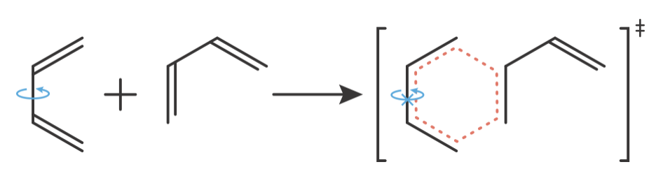
Figure 8.10: The Diels-Alder cycloaddition transition state illustrates why geometric constraints can produce more negative $\Delta S^\ddagger$ values than predicted by simple degree-of-freedom counting. Left: The diene reactant possesses internal rotational freedom (rotation arrow). Right: The transition state requires formation of a planar, cyclic six-membered ring structure (shown in red dashes). This geometric constraint restricts the internal rotational freedom present in the reactants, producing additional negative entropy contributions beyond those from simple translational and rotational degree-of-freedom changes. This explains why our estimated pre-exponential factor typically overestimates experimental values for Diels-Alder reactions.

These examples demonstrate that pre-exponential factors depend not only on the changes in translational and rotational degrees of freedom, but also on how transition state formation affects internal molecular motions such as rotation around single bonds.

The derivation of this expression for $k^\ddagger$ requires a statistical mechanical treatment of transition state theory. You will cover statistical mechanics in the third year of your course. A brief overview of the statistical formulation of transition state theory is given in Appendix D.↩︎
The statistical factor can equivalently be expressed as a configurational entropy contribution: $\Delta S^\ddagger_\mathrm{conf} = R \ln l$. This reflects the increased number of microstates available to the activated complex when multiple equivalent reaction pathways exist.↩︎