Lecture 3 Parallel Reversibile Reactions

3.1 Introduction to Parallel Reversible Reactions

Building on our previous discussion of parallel reactions, we now consider systems where the individual reactions are reversible:

\[\mathrm{A} \mathrel{\mathop{\rightleftarrows}^{k_1}_{k_{-1}}} \mathrm{B}\] \[\mathrm{A} \mathrel{\mathop{\rightleftarrows}^{k_2}_{k_{-2}}} \mathrm{C}\]

For such systems, the rate equations are:

\[\frac{\mathrm{d}[\mathrm{A}]}{\mathrm{d}t} = -(k_1 + k_2)[\mathrm{A}] + k_{-1}[\mathrm{B}] + k_{-2}[\mathrm{C}]\]

\[\frac{\mathrm{d}[\mathrm{B}]}{\mathrm{d}t} = +k_1[\mathrm{A}] - k_{-1}[\mathrm{B}]\]

\[\frac{\mathrm{d}[\mathrm{C}]}{\mathrm{d}t} = +k_2[\mathrm{A}] - k_{-2}[\mathrm{C}]\]

3.2 Time Evolution of Product Distributions

3.2.1 Short-Time Behaviour

At very short times, when [B] ≈ 0 and [C] ≈ 0, the backward reactions can be neglected and the system behaves similarly to the irreversible case we studied previously. The relative yields of products are determined by the ratio of the forward rate constants:

\[\frac{[\mathrm{B}]}{[\mathrm{C}]} \approx \frac{k_1}{k_2}\]

This is often called “kinetic control”, as the product distribution is determined by the relative rates of the forward reactions.

3.2.2 Long-Time Behaviour

At long times, the system reaches equilibrium, where:

\[\frac{\mathrm{d}[\mathrm{A}]}{\mathrm{d}t} = \frac{\mathrm{d}[\mathrm{B}]}{\mathrm{d}t} = \frac{\mathrm{d}d[\mathrm{C}]}{\mathrm{d}t} = 0\]

At equilibrium:

\[k_1[\mathrm{A}]_\mathrm{eq} = k_{-1}[\mathrm{B}]_\mathrm{eq}\] \[k_2[\mathrm{A}]_\mathrm{eq} = k_{-2}[\mathrm{C}]_\mathrm{eq}\]

This gives equilibrium constants:

\[K_\mathrm{AB} = \frac{[\mathrm{B}]_\mathrm{eq}}{[\mathrm{A}]_\mathrm{eq}} = \frac{k_1}{k_{-1}}\] \[K_\mathrm{AC} = \frac{[\mathrm{C}]_\mathrm{eq}}{[\mathrm{A}]_\mathrm{eq}} = \frac{k_2}{k_{-2}}\]

The final product ratio at equilibrium is:

\[\frac{[\mathrm{B}]_\mathrm{eq}}{[\mathrm{C}]_\mathrm{eq}} = \frac{k_1k_{-2}}{k_{-1}k_2}\]

This is called “thermodynamic control”, as the product distribution is determined by the relative thermodynamic stabilities of the products.

3.3 Kinetic vs Thermodynamic Control

When thinking about a pair of parallel reactions, we can rationalise a preference for forming either the kinetic or thermodynamic product by considering how the energy of a molecular system changes as reactants transform to products.

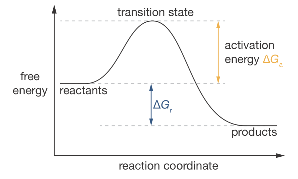
$A reaction coordinate diagram showing the free energy profile for a chemical reaction. The reaction coordinate represents the progression through molecular geometric changes (e.g., bonds breaking and forming) as reactants transform into products. The activation energy ($\Delta G_\mathrm{a}$) determines reaction rate, while the reaction free energy ($\Delta G_\mathrm{r}$) determines the position of equilibrium.$

Figure 3.1: A reaction coordinate diagram showing the free energy profile for a chemical reaction. The reaction coordinate represents the progression through molecular geometric changes (e.g., bonds breaking and forming) as reactants transform into products. The activation energy ($\Delta G_\mathrm{a}$) determines reaction rate, while the reaction free energy ($\Delta G_\mathrm{r}$) determines the position of equilibrium.

Figure 3.1 shows an example of a reaction coordinate diagram. A reaction coordinate diagram is a schematic representation of how the free energy of a molecular system changes as a reaction proceeds. The horizontal axis is called the reaction coordinate, and represents the progression of the reaction along a particular reaction pathway—often this corresponds to a specific change in geometry as atoms rearrange and bonds break and form. The vertical axis shows the Gibbs free energy of the system.

Two key features of these diagrams help us understand reaction behaviour:

The activation energy ($\Delta G_\mathrm{a}$) represents the energy barrier that must be overcome for reaction to occur. This determines reaction rate—lower barriers mean faster reactions.
The reaction free energy ($\Delta G_\mathrm{r}$) represents the overall thermodynamic driving force. This determines the position of equilibrium—more negative values mean the products are more favoured at equilibrium.

We can expand this concept of a reaction coordinate diagram to the case of parallel reactions by considering a diagram that shows two paths, A → B and A → C. In this composite reaction coordinate diagram, both paths start from the reactant A. One path leads to product B and the other path leads to product C. To understand the competition between kinetic and thermodymamic control, we consider the case where:

The reaction A → B has a lower activation energy than the reaction A → C;
C is thermodynamically favoured versus B; i.e., $\Delta G(B \to C) < 0$.

At short times, the concentrations of B and C are small, and relative concentrations of B and C approximately follow the relative rates of the corresponding forward reactions. Because the activation barrier for A → B is smaller than for A → C, B forms more rapidly than C, and [B]/[C] > 1. The kinetic product is therefore B.

At long times the kinetic product, B, can convert back to the reactant A, via path B → A, and then convert to C, via path A → C. Eventually we reach an equilibrium distribution of products, where the ratio [B]/[C] at equilibrium depends on the relative free energies of the two competing products. Because $\Delta G(B \to C) < 0$, at long times C is favoured (thermodynamic product) and [B]/[C] < 1.

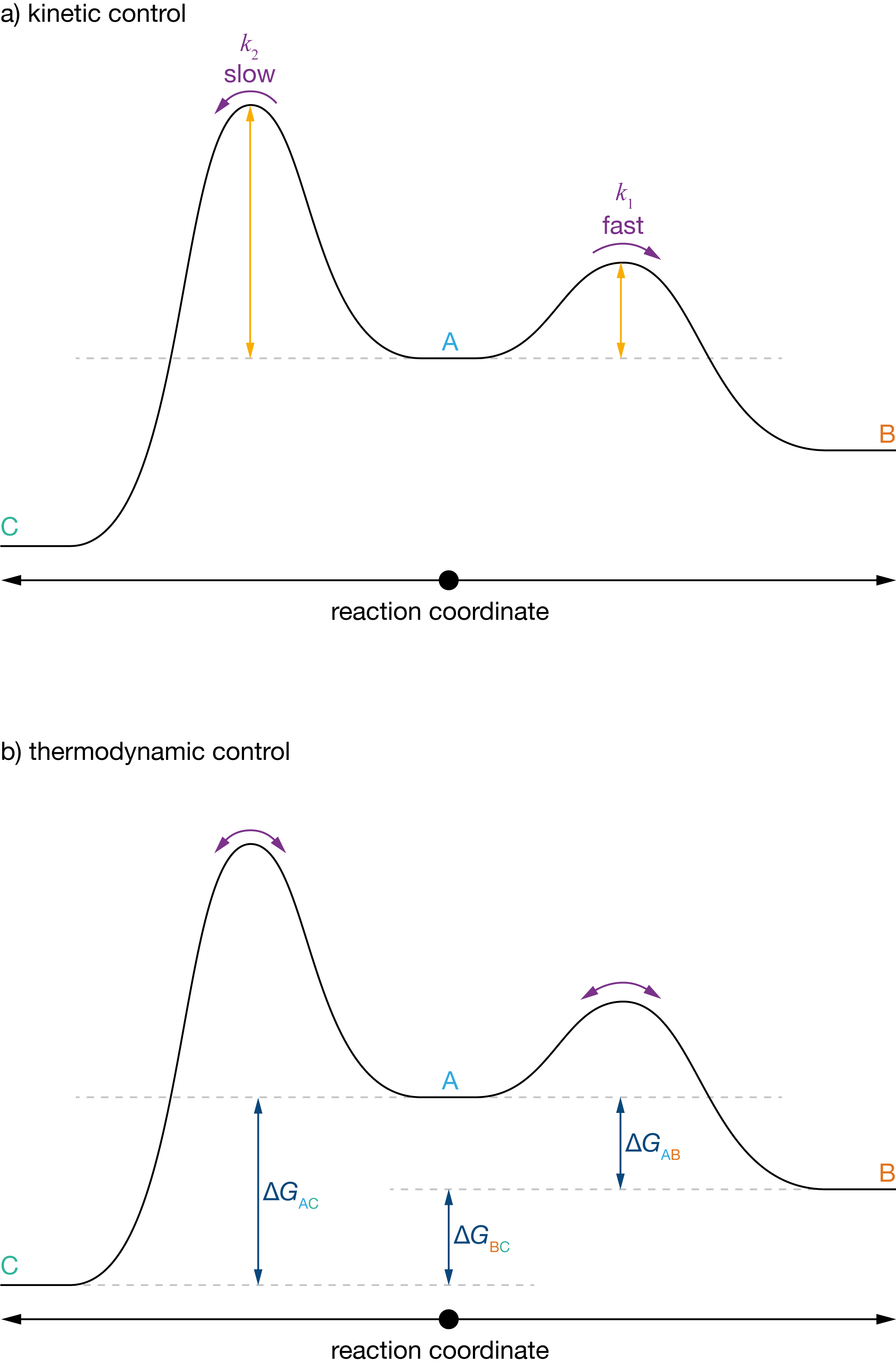
$Reaction coordinate diagram for a pair of parallel reversible reactions: A$\,\overset{k_1}{\underset{k_{-1}}\rightleftharpoons}\,$B and A$\,\overset{k_2}{\underset{k_{-2}}\rightleftharpoons}\,$C, where $\Delta E_1 < \Delta E_2$ (i.e., $k_1 \gg k_2$) and $\Delta G(\mathrm{B} \to \text{C}) < 0$. (a) kinetic control: at short times the relative formation of B and C depends only on the relative rates of the forward reactions A → B and A → C. (b) thermodynamic control: at long times the relative formation of B and C depends on the free energy difference between the two products.$

Figure 3.2: Reaction coordinate diagram for a pair of parallel reversible reactions: A$\,\overset{k_1}{\underset{k_{-1}}\rightleftharpoons}\,$B and A$\,\overset{k_2}{\underset{k_{-2}}\rightleftharpoons}\,$C, where $\Delta E_1 < \Delta E_2$ (i.e., $k_1 \gg k_2$) and $\Delta G(\mathrm{B} \to \text{C}) < 0$. (a) kinetic control: at short times the relative formation of B and C depends only on the relative rates of the forward reactions A → B and A → C. (b) thermodynamic control: at long times the relative formation of B and C depends on the free energy difference between the two products.

3.4 Example: Enolate formation of 2-methylcyclohexanone

Thinking about competing products as being preferentially formed under kinetic or thermodynamic control gives us a framework for understanding how our choice of reaction conditions can determine the selectivity of reaction. As an example, consider enolate formation of 2-methylcyclohexanone.

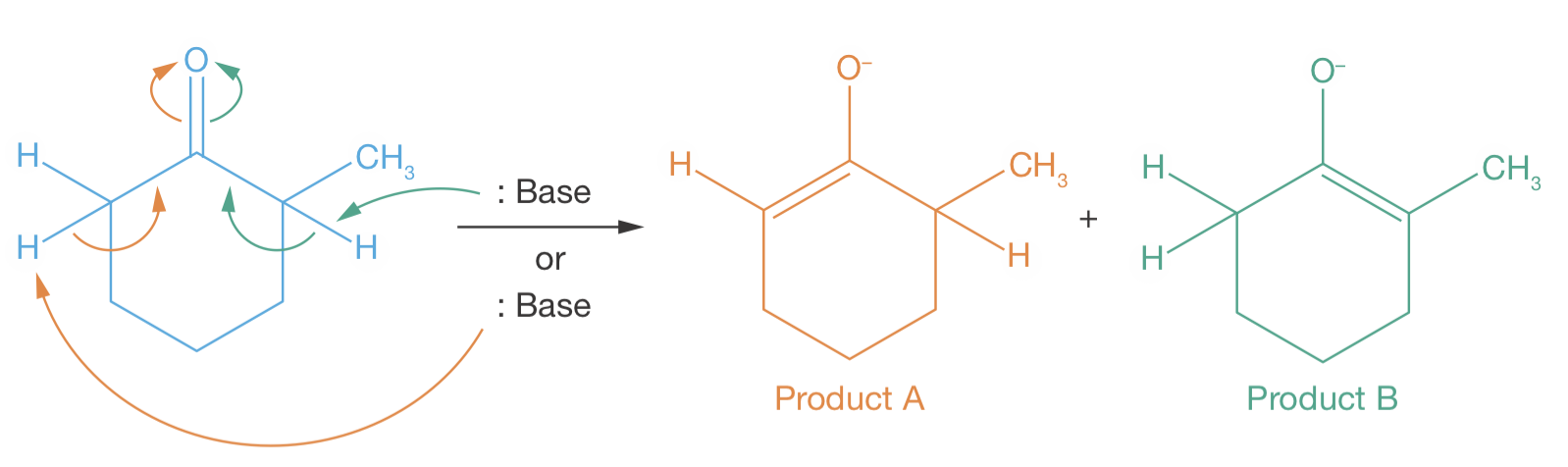
Under basic conditions, 2-methylcyclohexanone can form two distinct enolates, depending on whether a proton is removed from position 2 (green) or from position 6 (orange).

Figure 3.3: Under basic conditions, 2-methylcyclohexanone can form two distinct enolates, depending on whether a proton is removed from position 2 (green) or from position 6 (orange).

2-methylcyclohexanone can form two different enolates, depending on whether the base extracts a proton from position 2 or from position 6. In the presence of a strong base, the less substituted enolate (product A) is preferentially formed with high selectivity. While in the presence of a weak base, the more substituted enolate (product B) is preferentially formed with moderate selectivity (see Figure 3.3).

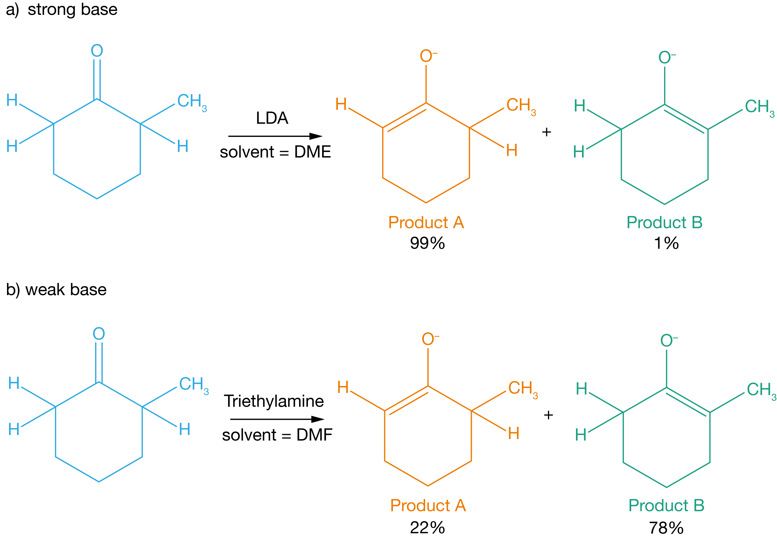
Figure 3.4: The selectivity between products A and B product B depends on the strength of the base that reacts with the 2-methylcyclohexanone.

We can understand the selectivity of this enolate formation, and why this depends on the strength of the base added, by thinking about the competition between the kinetic and thermodynamic products.

The thermodynamic product is the enolate that is thermodynamically more stable. In general, more subtituted alkenes are more stable than less substituted alkenes (see Figure 3.5), so we can expect product B to be the thermodynamic product.

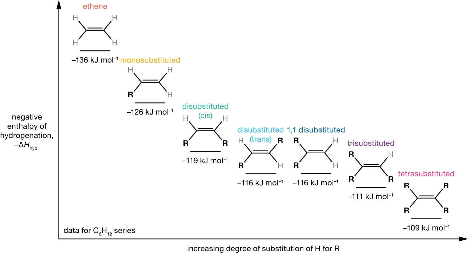
$Negative enthalpies of hydrogenation, $-\Delta H_\mathrm{hyd}$, for the series of C~6~H~12~ alkenes. The enthalpy of hydrogenation becomes less negative (less exothermic) as the degree of substitution of the alkene increases, indicating an increased stability of the C=C double bond.$

Figure 3.5: Negative enthalpies of hydrogenation, $-\Delta H_\mathrm{hyd}$, for the series of C₆H₁₂ alkenes. The enthalpy of hydrogenation becomes less negative (less exothermic) as the degree of substitution of the alkene increases, indicating an increased stability of the C=C double bond.

The kinetic product is the product that forms fastest at the start of the reaction, so to identify the kinetic product, we need to consider the relative rates of forward reactions, $k_\mathrm{A}$ and $k_\mathrm{B}$. Because of the methyl group at position 2, the proton at position 2 is sterically hindered, while the proton at position 6 is not. We can therefore expect the proton at position 6 to be removed more easily than the proton at position 2, with product A, therefore, formed faster than product B. Product A is the kinetic product.

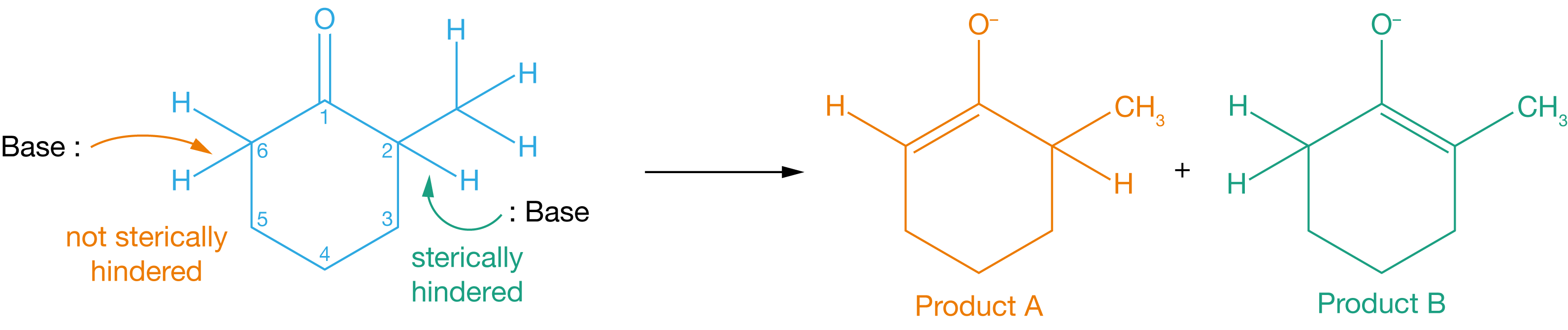
Removing the proton at position 6 gives product A, while removing the proton at position 2 gives product B. The proton at position 2 is more sterically hindered than the proton at position 6, so is harder to remove.

Figure 3.6: Removing the proton at position 6 gives product A, while removing the proton at position 2 gives product B. The proton at position 2 is more sterically hindered than the proton at position 6, so is harder to remove.

Now that we have identified the kinetic product as product A and the thermodynamic product as product B, we can think about why using a strong base gives predominantly product A (kinetic control) but a weak base gives predominantly product B (thermodynamic control).

First, let us consider the case of using a strong base. We have already identified that $k_\text{A} > k_\text{B}$, by considering which proton is more easily removed. In the presence of a strong base, we can also say that the position of equilibrium for both products ie expected to strongly favour the products, i.e., $K_\mathrm{A} \gg 1$ and $K_\mathrm{B} \gg 1$. For a reversible reaction the equilibrium constant is equal to the ratio of rate constants for the forward and reverse reactions, so:

\[\begin{equation} \frac{k_\mathrm{A}}{k_{-\mathrm{A}}} \gg 1 \qquad \frac{k_\mathrm{B}}{k_{-\mathrm{B}}} \gg 1. \end{equation}\]

Both reverse reactions, B → R and C → R, where R is the reactant, are much slower than the corresponding forward reactions, and so we can treat both reactions as effectively irreversible. At the start of the reaction, product A is formed much more quickly than product B, and the relative amounts of products A and B reflect the different rates of the two forward reactions. Hence, we obtain a very high selectivity for the kinetic product A.

We can also analyse the selectivity for product A over product B using a reaction coordinate diagram (Figure 3.7). Because $K_\mathrm{A} \gg 1$ and $K_\mathrm{B} \gg 1$, the free energies of formation of both products, A and B, are large (because $\Delta G_\mathrm{r} = -RT \ln K$). This means the barriers for the reverse reactions A → R and B → R are large, and these reverse reactions are very slow, making both reactions effectively irreversible. In addition, the barrier for R → A is lower than the barrier for R → B, so product A will form faster than product B. This combination of faster formation of A than of B and effective irreversibility of both reactions gives us strong selectivity for the kinetic product, A.

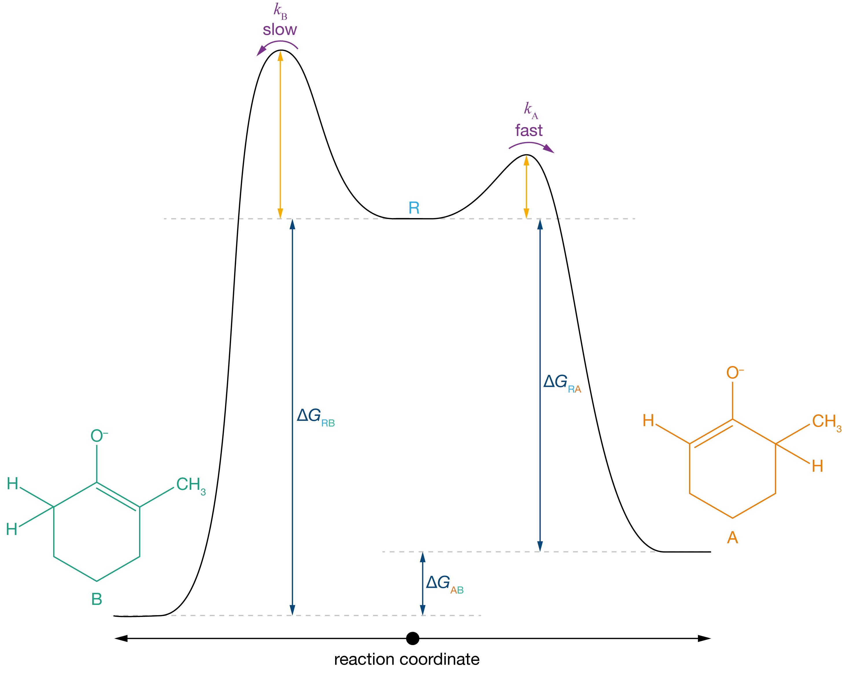
In the presence of a strong base, the position of equilibrium strongly favours both enolates, and both forward reactions are effectively irreversible. The pathway R → A has a lower activation barrier than the pathway R → B, so product A is formed faster than product B, resulting in strong selectivity for product A.

Figure 3.7: In the presence of a strong base, the position of equilibrium strongly favours both enolates, and both forward reactions are effectively irreversible. The pathway R → A has a lower activation barrier than the pathway R → B, so product A is formed faster than product B, resulting in strong selectivity for product A.

In the presence of a weak base, both equilibria are more balanced: $K_\mathrm{A} \approx 1$ and $K_\mathrm{B} \approx 1$. Again, using the fact that these equiibrium constants are equal to the ratios of rate constants for the forward and reverse reactions, this tells us that $k_{-\mathrm{A}} \approx k_\mathrm{A}$ and $k_{-\mathrm{B}} \approx k_\mathrm{B}$, i.e., both reverse reactions have rates that are approximately equal to the corresponding forward reactions, and are therefore highly reversible. We still have $k_\text{A} > k_\text{B}$, and, so, at the start of the reaction product A forms faster than product B. But, because R → A is reversible, A is able to convert back to the reactant and then to form product B. Eventually we end up with a ratio [B]/[A] that reflects the free energy difference between the two products, with preferential formation for the thermodynamic product, B.

In the presence of a weak base, the position of equilibrium less strongly favours both enolates, and both reactions are effectively reversible. Now the selectivity is determined by the free energy difference between the two products. Because B is more thermodymamically stable than A (because it is the more substituted enolate), we get preferential selectivity for the thermodynamic product B.

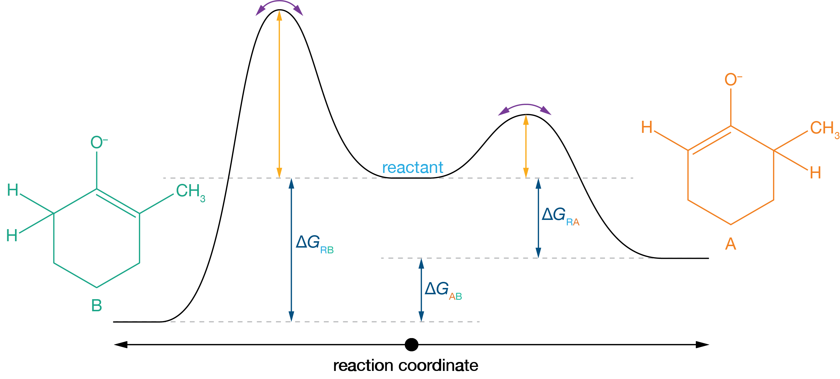
Figure 3.8: In the presence of a weak base, the position of equilibrium less strongly favours both enolates, and both reactions are effectively reversible. Now the selectivity is determined by the free energy difference between the two products. Because B is more thermodymamically stable than A (because it is the more substituted enolate), we get preferential selectivity for the thermodynamic product B.