Lecture 6 Transition State Theory
6.1 A Molecular Theory of Reaction Rates
Collision theory explains reaction rates using a simple model of colliding spheres. While this works for some gas-phase reactions, it cannot predict steric factors or explain systematic trends in activation energies. We need a more sophisticated approach.
For a reaction A + B → P, molecules must pass over an energy barrier before forming products. The reaction coordinate diagram shows this energy profile, from reactants through to products. The point at the highest point of the energy barrier is called the transition state; at this point the reacting molecules form a specific arrangement called the activated complex2, in which bonds are partially broken and new bonds are starting to form. Transition state theory provides a framework for analyzing this activated complex and using it to predict reaction rates.
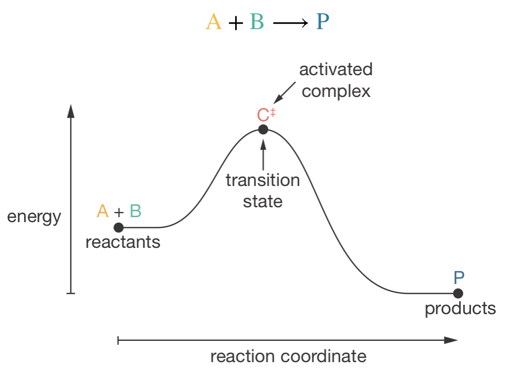
Figure 6.1: A reaction coordinate diagram for the reaction A + B → P. The energy profile shows the barrier that must be crossed as reactants are converted to products. The peak of this barrier corresponds to the transition state configuration, and the collection of molecules at the transition state form the activated complex, C\(^\ddagger\).
6.2 Basic Principles of Transition State Theory
Transition state theory treats the overall reaction A + B → P as occurring in two steps. First, the reactants A and B combine to form the activated complex C\(^{\ddagger}\). This complex can either fall apart back to reactants or go on to form products. The theory makes a key assumption: we can treat the activated complex as being in equilibrium with the reactants, even though C\(^{\ddagger}\) is inherently unstable. We call this a pseudo-equilibrium to reflect this special status.
The second step is the conversion of C\(^{\ddagger}\) to products, which we assume occurs with a characteristic rate constant \(k^{\ddagger}\). This is a first-order process — the rate depends only on the concentration of the activated complex:
\[\nu = \frac{\mathrm{d}[\mathrm{P}]}{\mathrm{d}t} = k^{\ddagger}[\mathrm{C}^{\ddagger}]\]
We can write the complete process as: \[\begin{equation} \mathrm{A} + \mathrm{B} \rightleftharpoons \mathrm{C}^{\ddagger} \xrightarrow{k^{\ddagger}} \mathrm{P} \tag{6.1} \end{equation}\]
6.3 Mathematical Development of Transition State Theory
To develop our rate equation, we begin by considering the pseudo-equilibrium between reactants and the activated complex. We can define a pseudo-equilibrium constant:
\[\begin{equation} K^{\ddagger} = \frac{[\mathrm{C}^{\ddagger}]c^\circ}{[\mathrm{A}][\mathrm{B}]} \tag{6.2} \end{equation}\]
where \(c^\circ\) = 1 mol dm−3 is the standard concentration.3
This allows us to express the concentration of the activated complex in terms of reactant concentrations:
\[\begin{equation} [\mathrm{C}^{\ddagger}] = (K^{\ddagger}/c^\circ)[\mathrm{A}][\mathrm{B}] \tag{6.3} \end{equation}\]
Since we treat the formation of the activated complex as a pseudo-equilibrium, we can apply standard thermodynamic relationships. The equilibrium constant \(K^{\ddagger}\) relates to the activation Gibbs energy through:
\[\begin{equation} \Delta G^{\ddagger} = -RT\ln(K^{\ddagger}) \tag{6.4} \end{equation}\]
We can then use the standard relationship \(\Delta G^\ddagger = \Delta H^\ddagger - T \Delta S^\ddagger\) to separate \(K^\ddagger\) into enthalpic and entropic terms:
\[\begin{equation} K^{\ddagger} = \mathrm{e}^{-\Delta G^{\ddagger}/RT} = \mathrm{e}^{-\Delta H^{\ddagger}/RT}\mathrm{e}^{\Delta S^{\ddagger}/R} \tag{6.5} \end{equation}\]
From our second assumption, the rate of product formation is proportional to the concentration of the activated complex:
\[\begin{equation} \nu = k^{\ddagger}[\mathrm{C}^{\ddagger}] = \frac{k^{\ddagger}}{c^{\circ}}[\mathrm{A}][\mathrm{B}]\mathrm{e}^{\Delta S^{\ddagger}/R}\mathrm{e}^{-\Delta H^{\ddagger}/RT} \tag{6.6} \end{equation}\]
This expression is known as the Eyring equation, and has the form of a second-order rate law with rate constant:
\[\begin{equation} k = \frac{k^{\ddagger}}{c^{\circ}}\mathrm{e}^{\Delta S^{\ddagger}/R}\mathrm{e}^{-\Delta H^{\ddagger}/RT} \tag{6.7} \end{equation}\]
6.4 Relationship to the Arrhenius Equation
We can understand how transition state theory connects to experimental observations by comparing the rate constant expression with the Arrhenius equation:
From transition state theory: \[\begin{equation} k = \frac{k^{\ddagger}}{c^{\circ}}\mathrm{e}^{\Delta S^{\ddagger}/R}\mathrm{e}^{-\Delta H^{\ddagger}/RT} \tag{6.8} \end{equation}\]
The Arrhenius equation: \[\begin{equation} k = A\mathrm{e}^{-E_\mathrm{a}/RT} \tag{5.5} \end{equation}\]
This comparison reveals two important correspondences:
- The activation enthalpy \(\Delta H^{\ddagger}\) plays a similar role to the Arrhenius activation energy \(E_\mathrm{a}\).
- The pre-exponential factor \(A\) corresponds to \(\frac{k^{\ddagger}}{c^{\circ}}\mathrm{e}^{\Delta S^{\ddagger}/R}\).
Like collision theory, transition state theory provides a molecular-level interpretation of the Arrhenius parameters. However, transition state theory offers additional insight by separating the activation barrier into enthalpic (\(\Delta H^{\ddagger}\)) and entropic (\(\Delta S^{\ddagger}\)) contributions, helping explain systematic variations in reactivity across related compounds.
6.5 Enthalpy of Activation
The enthalpy of activation \(\Delta H^{\ddagger}\) represents the enthalpic contribution to forming the activated complex. For a simple reaction where C breaks an A–B bond to form B–C, examining what happens at the transition state reveals why this enthalpy change varies systematically between related reactions.
In the activated complex, the original A–B bond is almost completely broken, while the new B–C bond has only started to form. This means \(\Delta H^{\ddagger}\) depends primarily on the strength of the bond being broken. The strength of the bond being formed has much less effect, since this bond is still weak in the transition state.
This principle helps explain trends in activation energies for a family of related reactions. Consider these examples involving H and Br:
\[\begin{align*} \mathrm{H–H} + \mathrm{H} &\longrightarrow \mathrm{H} + \mathrm{H–H} & E_\mathrm{a} &= +39~\mathrm{kJ~mol^{-1}} \\ \mathrm{H–H} + \mathrm{Br} &\longrightarrow \mathrm{H} + \mathrm{H–Br} & E_\mathrm{a} &= +82~\mathrm{kJ~mol^{-1}} \\ \mathrm{Br–H} + \mathrm{H} &\longrightarrow \mathrm{Br} + \mathrm{H–H} & E_\mathrm{a} &= +12~\mathrm{kJ~mol^{-1}} \\ \mathrm{Br–Br} + \mathrm{H} &\longrightarrow \mathrm{Br} + \mathrm{Br–H} & E_\mathrm{a} &= +4~\mathrm{kJ~mol^{-1}} \end{align*}\]
To understand these trends, we need to consider the bond dissociation energies:
\[\begin{align*} \mathrm{H–H}: & ~E_\mathrm{d} = +436~\mathrm{kJ~mol^{-1}} \\ \mathrm{H–Br}: & ~E_\mathrm{d} = +366~\mathrm{kJ~mol^{-1}} \\ \mathrm{Br–Br}: & ~E_\mathrm{d} = +193~\mathrm{kJ~mol^{-1}} \end{align*}\]
The trends in activation energy can be explained by:
- The first two reactions involve breaking H–H bonds (highest \(E_\mathrm{d}\)) → highest \(E_\mathrm{a}\) values
- Between these two:
- H–H + H forms H–H (more favorable)
- H–H + Br forms H–Br (less favorable)
- Therefore \(E_\mathrm{a}\) is lower for H–H + H
- The remaining reactions follow the trend in bond strength being broken:
- Breaking H–Br (\(E_\mathrm{a} = +12~\mathrm{kJ~mol^{-1}}\))
- Breaking Br–Br (\(E_\mathrm{a} = +4~\mathrm{kJ~mol^{-1}}\))
6.6 Reconciling Transition State Theory with Collision Theory
At first glance, Collision theory and transition state theory can seem to give different pictures of activation energy. In collision theory, \(E_\mathrm{a}\) represents a minimum kinetic energy molecules must have to react. In transition state theory, \(\Delta H^{\ddagger}\) represents the energy needed to distort and partially break bonds bonds in the activated complex.
We can connect these views by following the energy through a reactive collision. Initially, the molecules approach with kinetic energy at least equal to \(E_\mathrm{a}\). As they collide, this kinetic energy transforms into potential energy, with the molecular geometry distorting to form the activated complex. Here, the initial kinetic energy has become the energy stored in partially broken and formed bonds — our \(\Delta H^{\ddagger}\). By energy conservation, these energies must be approximately equal.
The two theories thus describe the same process from different perspectives: collision theory focuses on the keinetic energy molecules must have before they collide, while transition state theory considers how this energy is used in making and breaking bonds.
6.7 Entropy of Activation
We have seen that transition state theory provides a molecular interpretation of the Arrhenius pre-exponential factor \(A\) in terms of an entropy of activation \(\Delta S^{\ddagger}\). To understand what this entropy term means and what determines its magnitude, we need to think carefully about what entropy means at a molecular level.
6.7.1 Understanding Molecular Entropy
While entropy is often simply described as a measure of “disorder”, this description can be misleading. For many chemical reactions, simple arguments based on relative “disorder” fail to predict even qualitative behaviour. This becomes particularly apparent when considering gas-phase reactions: both reactants and products exist as freely moving molecules, so which state is more “disordered”?
A more useful framework considers entropy in terms of molecular freedom and statistical likelihood. Systems with greater freedom have higher entropy than more constrained systems, and molecular arrangements that are statistically more likely have higher entropy than less likely arrangements.
The spontaneous expansion of an ideal gas illustrates these ideas. An ideal gas expands to fill its container despite no change in internal energy (\(\Delta U = 0\)) or enthalpy (\(\Delta H = 0\), since \(pV = nRT\)). This process occurs spontaneously because the expanded state has higher entropy: gas molecules have more freedom to move through a larger volume, and an even distribution throughout the available space is statistically more likely than having all molecules confined to a smaller region.
6.7.2 Entropy of Activation for Bimolecular Reactions
For a gas-phase bimolecular reaction, forming the activated complex introduces new constraints on molecular motion:
\[\mathrm{A} + \mathrm{B} \rightleftharpoons \mathrm{C}^{\ddagger}\]
Each molecule in the gas phase has three translational degrees of freedom—the molecules are free to move along the \(x\), \(y\), and \(z\) axes, independently of the motion of the other molecules in the system. The reactants A and B therefore have six translational degrees of freedom between them. When these molecules combine to form the activated complex, however, we have just three translational degrees of freedom, since \(\mathrm{C}^{\ddagger}\) moves as a single unit through space. This loss of translational freedom corresponds to a decrease in entropy. For gas-phase bimolecular reactions, \(\Delta S^{\ddagger}\) is therefore always negative, reflecting the increased constraints imposed when forming the activated complex.
In our treatment using 2D reaction coordinate diagrams, we represent the transition state as a single point at the peak of the energy barrier. In reality, for a molecular system with many degrees of freedom, the transition state is a dividing surface on the multidimensional potential energy surface. The “activated complex” comprises all molecular configurations on this dividing surface.↩︎
Many basic treatments of transition state theory omit \(c^{\circ}\) since it equals 1 under standard conditions. Including it ensures that \(K^\ddagger\) is correctly defined as dimensionless, and that \(k\) has the correct units for a second-order rate constant of dm\(^3\) mol\(^{-1}\) s\(^{-1}\).↩︎