Lecture 5 Collision Theory

5.1 Introduction to Kinetic Theories

Up to this point, we have focused on describing and interpreting empirical data—either deriving rate laws from experimental data or proposing reaction mechanisms and comparing their predictions against observations. While this approach allows us to understand the shape of concentration–time profiles, it does not explain quantitative differences in reaction rates.

Several important questions remain: - For two bimolecular reactions, which would we expect to be faster, and by how much? - Can we predict rate constants $k$ (and how they vary with temperature) without experimental data?

While we have discussed the Arrhenius equation, $k = A_0\mathrm{e}^{-\Delta E/RT}$, this is an approximate empirical relationship that requires experimental data to determine $A_0$ and $\Delta E$. To move beyond empirical descriptions, we need microscopic theories that can make quantitative predictions of reaction rates.

In this course, we will examine two such theories:

Collision Theory (this lecture)—focuses on gas-phase bimolecular reactions, treating molecules as hard spheres
Transition State Theory (lectures 6–9)—considers formation of activated complexes for all types of reactions

5.2 Fundamentals of Collision Theory

Collision theory provides one of the simplest microscopic models of reaction rates, specifically for gas-phase bimolecular reactions of the form:

\[\mathrm{A} + \mathrm{B} \rightarrow \mathrm{P}\]

For such reactions, we expect a rate law of the form $\nu = k[\mathrm{A}][\mathrm{B}]$, but what determines the value of $k$?

5.2.1 Basic Principles and Assumptions

Building on the kinetic theory of gases, collision theory makes two key assumptions:

Molecules behave as hard spheres
Molecules must collide to react

The overall reaction rate is then:

rate = rate of collisions × fraction of “successful” collisions

5.2.2 Collision Frequency

To determine the rate of collisions, we need to calculate how often molecules A and B encounter each other in the gas phase. Consider two molecules with radii $r_\mathrm{A}$ and $r_\mathrm{B}$ moving with velocities $v_\mathrm{A}$ and $v_\mathrm{B}$.

We can simplify this problem by working in the reference frame of molecule A, where A appears stationary and B molecules move with the relative velocity $v = |v_\mathrm{B} - v_\mathrm{A}|$.

A collision occurs when the centres of the two molecules come within a distance $d = r_\mathrm{A} + r_\mathrm{B}$ of each other. As shown in Figure 5.1, molecule A (green) can be thought of as sitting at the centre of a cylindrical “target zone”. Any molecule B (orange) whose centre lies within this cylinder will collide with A.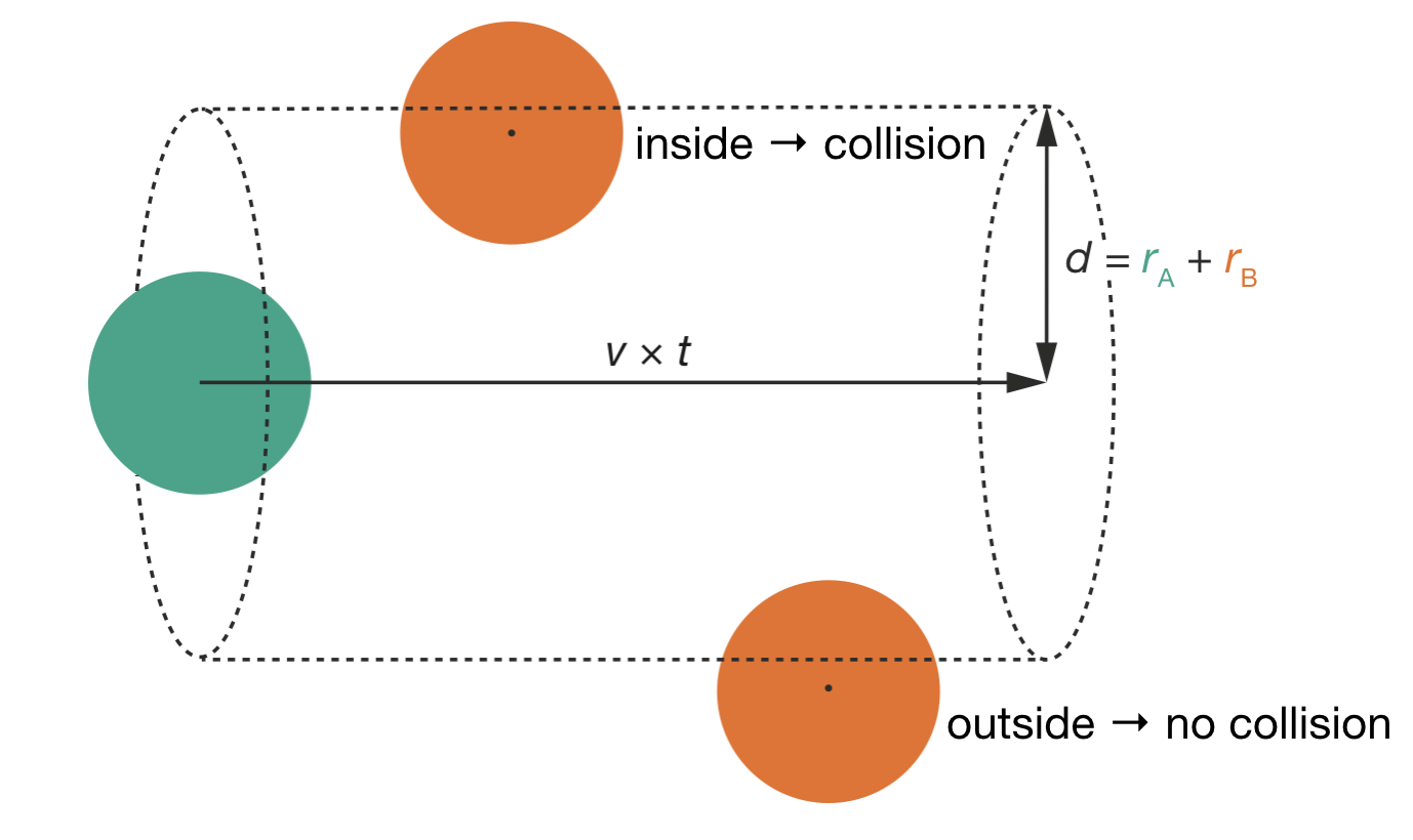

$Collision geometry in the reference frame of molecule A. Molecule A (teal) sits at the centre of a cylindrical volume of radius $d = r_\mathrm{A} + r_\mathrm{B}$ (shown as dashed outline). As time progresses by $t$, this cylinder extends by length $v \times t$, where $v$ is the relative velocity. Molecules B (orange) with centres inside this cylinder will collide with A; those outside will not.$

Figure 5.1: Collision geometry in the reference frame of molecule A. Molecule A (teal) sits at the centre of a cylindrical volume of radius $d = r_\mathrm{A} + r_\mathrm{B}$ (shown as dashed outline). As time progresses by $t$, this cylinder extends by length $v \times t$, where $v$ is the relative velocity. Molecules B (orange) with centres inside this cylinder will collide with A; those outside will not.

The dimensions of this collision cylinder are:

Radius = $d = (r_\mathrm{A} + r_\mathrm{B})$
Cross-sectional area = $S = \pi d^2$
Length swept in time $t$ = $vt$ (where $v$ is the relative velocity)
Volume swept in time $t$ = $vt \times \pi d^2$

The volume swept per unit time is therefore $v\pi d^2$. Any molecule B whose centre lies within this volume will collide with molecule A. If there are $N_\mathrm{B}$ molecules of B in total volume $V$, the number of B molecules per unit volume is $N_\mathrm{B}/V$, and the number of collisions that one molecule A makes per unit time is:

\[\frac{N_\mathrm{B}}{V}v\pi d^2\]

To find the total collision frequency per unit volume, we multiply by the concentration of A molecules. This gives the collision frequency per unit volume ($Z'$):

\[Z' = \frac{N_\mathrm{A}N_\mathrm{B}}{V^2}v\pi d^2\]

where $N_\mathrm{A}$ and $N_\mathrm{B}$ are the total numbers of molecules of each species in volume $V$.

5.2.3 Average Relative Velocity

In our expression for collision frequency, we used the relative velocity $v$ between molecules A and B. However, in a gas at temperature $T$, molecules have a distribution of velocities—not all molecules move at the same speed. To calculate the collision frequency, we need the average relative velocity.

From the kinetic theory of gases, the average relative velocity between molecules A and B depends on both temperature and the reduced mass of the colliding pair. The reduced mass $\mu$ is defined as:

\[\mu = \frac{m_\mathrm{A}m_\mathrm{B}}{m_\mathrm{A} + m_\mathrm{B}}\]

The average relative velocity is then:

\[\langle v \rangle = \left(\frac{8k_\mathrm{B}T}{\pi\mu}\right)^{1/2}\]

This expression shows that:

Lighter molecules (smaller $\mu$) move faster on average and collide more frequently
Higher temperatures increase molecular speeds and collision rates
The velocity increases with the square root of temperature

Substituting this average velocity into our collision frequency expression gives:

\[Z' = \frac{N_\mathrm{A}N_\mathrm{B}}{V^2}\pi d^2\left(\frac{8k_\mathrm{B}T}{\pi\mu}\right)^{1/2}\]

This is the collision frequency per unit volume for molecules A and B in a gas at temperature $T$.

5.3 From Collisions to Reaction Rates

5.3.1 Energetic Requirements for Reaction

Not every collision between molecules A and B leads to reaction. The collision frequency $Z'$ tells us how often molecules encounter each other, but only a fraction of these collisions have sufficient energy to overcome the activation barrier and form products.

In collision theory, we assume that molecules must possess a minimum relative kinetic energy $E_\mathrm{a}$ (the activation energy) for reaction to occur. This threshold energy is needed to break bonds and rearrange atoms during the collision. The question then becomes: what fraction of molecular collisions have relative kinetic energy greater than or equal to $E_\mathrm{a}$?

The answer comes from the Maxwell-Boltzmann distribution of molecular speeds. In a gas at temperature $T$, the relative kinetic energies of colliding molecules follow a probability distribution that depends on temperature, as shown in Figure 5.2.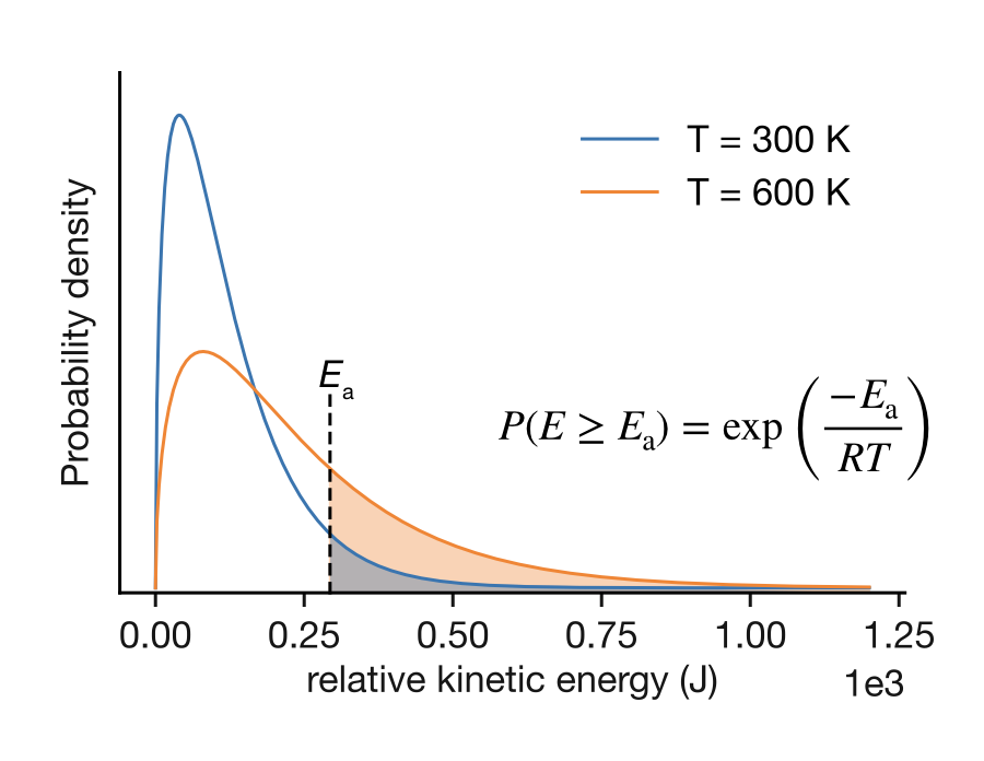

$Maxwell-Boltzmann distribution of relative kinetic energies for molecular collisions at two temperatures. The shaded regions show the fraction of collisions with energy $E \geq E_\mathrm{a}$. At higher temperature (orange, 600 K), the distribution broadens and shifts to higher energies, increasing the fraction of collisions with sufficient energy to react. The fraction of successful collisions is given by $P(E \geq E_\mathrm{a}) = \exp(-E_\mathrm{a}/RT)$.$

Figure 5.2: Maxwell-Boltzmann distribution of relative kinetic energies for molecular collisions at two temperatures. The shaded regions show the fraction of collisions with energy $E \geq E_\mathrm{a}$. At higher temperature (orange, 600 K), the distribution broadens and shifts to higher energies, increasing the fraction of collisions with sufficient energy to react. The fraction of successful collisions is given by $P(E \geq E_\mathrm{a}) = \exp(-E_\mathrm{a}/RT)$.

The figure shows two key features:

Temperature dependence: At higher temperature (orange curve, 600 K), the distribution is broader and shifted to higher energies compared to lower temperature (blue curve, 300 K). This means a larger fraction of collisions have energy exceeding $E_\mathrm{a}$.
Exponential tail: The shaded region represents collisions with $E \geq E_\mathrm{a}$. The fraction of collisions in this high-energy tail follows directly from the kinetic theory of gases :¹

\[P(E \geq E_\mathrm{a}) = \exp\left(-\frac{E_\mathrm{a}}{RT}\right)\]

5.3.2 The Complete Rate Expression

Combining the collision frequency with the probability that a collision has sufficient energy, we obtain:

\[\text{rate} = Z' \times P(E \geq E_\mathrm{a})\]

Substituting our expressions for $Z'$ and $P(E \geq E_\mathrm{a})$ gives:

\[\text{rate} = \frac{N_\mathrm{A}N_\mathrm{B}}{V^2}\pi d^2\left(\frac{8k_\mathrm{B}T}{\pi\mu}\right)^{1/2}\exp\left(-\frac{E_\mathrm{a}}{RT}\right)\]

To express this in the familiar form of a rate law, we convert from numbers of molecules to concentrations. The concentration of A is $[\mathrm{A}] = N_\mathrm{A}/V$ and similarly $[\mathrm{B}] = N_\mathrm{B}/V$, giving:

\[\text{rate} = \pi d^2\left(\frac{8k_\mathrm{B}T}{\pi\mu}\right)^{1/2}\exp\left(-\frac{E_\mathrm{a}}{RT}\right)[\mathrm{A}][\mathrm{B}]\]

This has exactly the form we expect for a bimolecular elementary reaction:

\[\begin{equation} \text{rate} = k[\mathrm{A}][\mathrm{B}] \end{equation}\]

where the rate is first-order with respect to A, first-order with respect to B, and second-order overall. The rate constant predicted by collision theory is:

\[\begin{equation} k = \pi d^2\left(\frac{8k_\mathrm{B}T}{\pi\mu}\right)^{1/2}\exp\left(-\frac{E_\mathrm{a}}{RT}\right) \tag{5.1} \end{equation}\]

This expression shows how collision theory connects the macroscopic rate constant to microscopic molecular properties: the collision cross-section ($\pi d^2$), the molecular masses (through $\mu$), the temperature, and the activation energy.

5.3.3 The Steric Factor

Our collision theory expression predicts that the rate constant should be:

\[k = \pi d^2\left(\frac{8k_\mathrm{B}T}{\pi\mu}\right)^{1/2}\exp\left(-\frac{E_\mathrm{a}}{RT}\right)\]

When we compare this theoretical prediction with experimental measurements, we find a systematic discrepancy: collision theory typically overestimates reaction rates, sometimes by several orders of magnitude. This tells us that our model of molecules as hard spheres is too simple—there is something missing from our picture of how molecules react.

To account for this discrepancy, we introduce an empirical correction factor $P$, called the steric factor. The steric factor is defined as the ratio of the experimentally measured pre-exponential factor to the theoretical value predicted by collision theory:

\[\begin{equation} P = \frac{A_\mathrm{exp}}{A_\mathrm{th}} \tag{5.2} \end{equation}\]

where $A_\mathrm{exp}$ comes from fitting the Arrhenius equation to experimental data, and $A_\mathrm{th} = \pi d^2\sqrt{8k_\mathrm{B}T/(\pi\mu)}$ is the pre-exponential factor predicted by collision theory.

By including the steric factor, we obtain a revised expression for the rate constant, $k$:

\[\begin{equation} k = P\pi d^2\left(\frac{8k_\mathrm{B}T}{\pi\mu}\right)^{1/2}\exp\left(-\frac{E_\mathrm{a}}{RT}\right) \tag{5.3} \end{equation}\]

Table 5.1 shows experimental pre-exponential factors, collision theory predictions, and the resulting steric factors for several representative reactions.

Table 5.1: Comparison of experimental and theoretical pre-exponential factors for representative bimolecular gas-phase reactions. The steric factor $P = A_\mathrm{exp}/A_\mathrm{th}$ quantifies how much collision theory overestimates ($P < 1$) or underestimates ($P > 1$) the reaction rate.
Reaction	$A_\mathrm{exp}$ / 10$^{11}$ dm$^3$ mol$^{-1}$ s$^{-1}$	$A_\mathrm{th}$ / 10$^{11}$ dm$^3$ mol$^{-1}$ s$^{-1}$	$P$
K + Br$_2$ $\rightarrow$ KBr + Br	10	2.1	4.8
CH$_3$ + CH$_3$ $\rightarrow$ C$_2$H$_6$	0.24	1.1	0.22
2NOCl $\rightarrow$ 2NO + Cl$_2$	0.094	0.59	0.16
H$_2$ + C$_2$H$_4$ $\rightarrow$ C$_2$H$_6$	1.24 $\times$ 10$^{-5}$	7.3	1.7 $\times$ 10$^{-6}$

The data in Table 5.1 show two key features. First, for most reactions, collision theory overestimates the reaction rate. The reaction 2NOCl → 2NO + Cl₂ has $P = 0.16$, meaning the experimental rate is only about one-sixth of the collision theory prediction. Second, the steric factor decreases systematically as molecular complexity increases. For methyl radical combination we find $P = 0.22$, while for the hydrogenation of ethene, $P = 1.7 ^{-6}—a difference of five orders of magnitude.

5.3.4 Physical Interpretation

We can interpret these observations in terms of molecular orientation requirements. For a reaction to occur, it is not sufficient for the reactants to have sufficient relative kinetic energy—molecules must also come together in specific orientations. The steric factor $P$ can be interpreted as representing how likely it is that a collision occurs with a geometry suitable for reaction. This interpretation explains why collision theory typically overestimates reaction rates: most collisions, even those with sufficient energy, involve unsuitable orientations.

With this interpretation of the steric factor, we can understand the systematic decrease in $P$ with molecular complexity as reflecting increasingly stringent geometric constraints. For larger, more complex molecules, only a small fraction of all possible collision orientations have the correct geometry for reaction. The hydrogenation of ethene provides an extreme example: H₂ must approach the C=C electron density in a specific orientation and cannot react if blocked by the CH₂ end-groups, leading to $P = 1.7 \times 10^{-6}$.

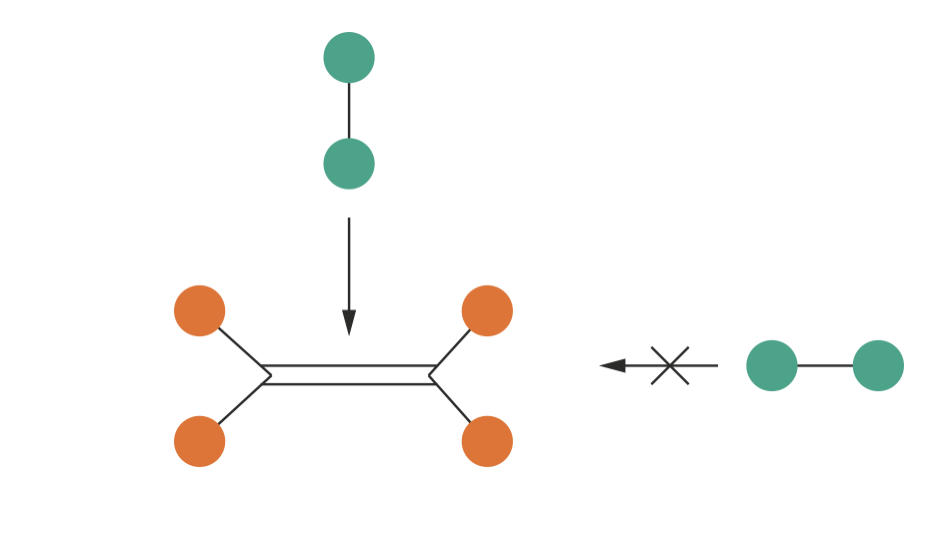
$Geometric constraints in the hydrogenation of ethene. H$_2$ (green) must approach the C=C double bond from above (arrow shows allowed approach) to react. Approach from the side is blocked by the CH$_2$ groups, preventing reaction even if the collision has sufficient energy. This stringent geometric requirement leads to $P = 1.7 \times 10^{-6}$.$

Figure 5.3: Geometric constraints in the hydrogenation of ethene. H$_2$ (green) must approach the C=C double bond from above (arrow shows allowed approach) to react. Approach from the side is blocked by the CH$_2$ groups, preventing reaction even if the collision has sufficient energy. This stringent geometric requirement leads to $P = 1.7 \times 10^{-6}$.

While this general principle explains the data where $P < 1$, the K + Br₂ reaction appears to contradict our conceptual model. Here, $P = 4.8$—reactions occur more frequently than collision theory predicts. This enhanced reactivity arises from the “harpoon mechanism”: during the approach of K and Br₂, an electron can transfer from potassium to bromine at relatively large separation, creating K⁺ and Br₂⁻ ions. The resulting electrostatic attraction pulls the reactants together and effectively increases the collision cross-section beyond what we would predict from hard-sphere radii. This demonstrates that our simple hard-sphere model can fail in both directions—it can underestimate rates when long-range forces are important, just as it typically overestimates rates when orientation constraints matter.

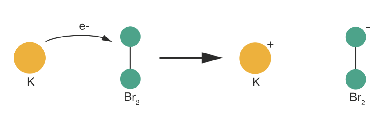
The harpoon mechanism in the K + Br$_2$ reaction. During approach, an electron transfers from potassium to bromine at relatively large separation, creating K$^+$ and Br$_2^-$ ions. The resulting electrostatic attraction increases the effective collision cross-section beyond what hard-sphere radii predict.

Figure 5.4: The harpoon mechanism in the K + Br$_2$ reaction. During approach, an electron transfers from potassium to bromine at relatively large separation, creating K$^+$ and Br$_2^-$ ions. The resulting electrostatic attraction increases the effective collision cross-section beyond what hard-sphere radii predict.

5.4 Relationship to the Arrhenius Equation

The rate constant derived from collision theory has a similar form to the empirical Arrhenius equation.

From collision theory: \[\begin{equation} k = P\pi d^2\left(\frac{8k_\mathrm{B}T}{\pi\mu}\right)^{1/2}\exp\left(-\frac{E_\mathrm{a}}{RT}\right) \tag{5.4} \end{equation}\]

The Arrhenius equation: \[\begin{equation} k = A_0\exp\left(-\frac{E_\mathrm{a}}{RT}\right) \tag{5.5} \end{equation}\]

This comparison provides physical insight into the meaning of the Arrhenius parameters:

The activation energy $E_\mathrm{a}$ in the Arrhenius equation can be interpreted as the minimum relative kinetic energy that colliding molecules must possess for reaction to occur. This threshold energy is needed to overcome the potential energy barrier to reaction.
The pre-exponential factor $A_0$ represents a normalized collision frequency. The collision theory expression shows that this frequency depends on:

The collision cross-section ($\pi d^2$)
The average relative velocity of molecules ($\propto \sqrt{T/\mu}$)
A steric factor $P$ that accounts for orientation requirements

Therefore, while the Arrhenius equation was originally proposed as an empirical relationship, collision theory provides a theoretical foundation for its functional form and offers molecular-level interpretations of its parameters. However, we should note that this interpretation is strictly valid only for gas-phase bimolecular reactions. For more complex reactions, particularly in solution, the physical meaning of the Arrhenius parameters becomes less clear, and we need more sophisticated theories to understand their molecular basis.

5.5 Limitations of Collision Theory as a Predictive Framework

Collision theory works reasonably well for simple molecules but typically overestimates reaction rates for complex molecules.

Two key limitations prevent collision theory from serving as a fully predictive framework:

The activation energy E$\mathrm{a}$ appears as an arbitrary “threshold energy” that molecules must possess to react. While we can measure this energy experimentally, the theory provides no insight into how $E_\mathrm{a}$ varies between different reactions.
While we can determine the steric factor $P$ by comparing experimental and theoretical rate constants, we have no quantitative theory to predict its value. This means we cannot predict absolute rate constants for new reactions without experimental data.

The derivation of this result from the Maxwell-Boltzmann distribution is given in Appendix B.↩︎

Reaction	\(A_\mathrm{exp}\) / 10\(^{11}\) dm\(^3\) mol\(^{-1}\) s\(^{-1}\)	\(A_\mathrm{th}\) / 10\(^{11}\) dm\(^3\) mol\(^{-1}\) s\(^{-1}\)	\(P\)
K + Br\(_2\) \(\rightarrow\) KBr + Br	10	2.1	4.8
CH\(_3\) + CH\(_3\) \(\rightarrow\) C\(_2\)H\(_6\)	0.24	1.1	0.22
2NOCl \(\rightarrow\) 2NO + Cl\(_2\)	0.094	0.59	0.16
H\(_2\) + C\(_2\)H\(_4\) \(\rightarrow\) C\(_2\)H\(_6\)	1.24 \(\times\) 10\(^{-5}\)	7.3	1.7 \(\times\) 10\(^{-6}\)