Lecture 1 Chemical Kinetics

1.1 Why Study Chemical Kinetics?

Chemical kinetics describes how reactions happen. While thermodynamics tells us whether a reaction will occur and what the final state will be, kinetics reveals how fast it happens and what steps are involved.

For any reaction A $\longrightarrow$ B, kinetics lets us predict how much B we’ll have after a given time, or how long we need to wait for a desired yield. Beyond this, understanding kinetics helps us control and optimize reactions by changing conditions like temperature and pressure.

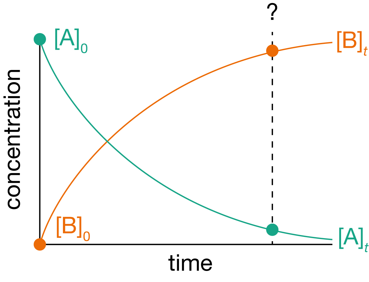
$A plot of concentrations of reactant A and product B for a generic reaction A $\longrightarrow$ B as a function of time. Over time, A is converted to B. How long will it take to obtain 90% yield?$

Figure 1.1: A plot of concentrations of reactant A and product B for a generic reaction A $\longrightarrow$ B as a function of time. Over time, A is converted to B. How long will it take to obtain 90% yield?

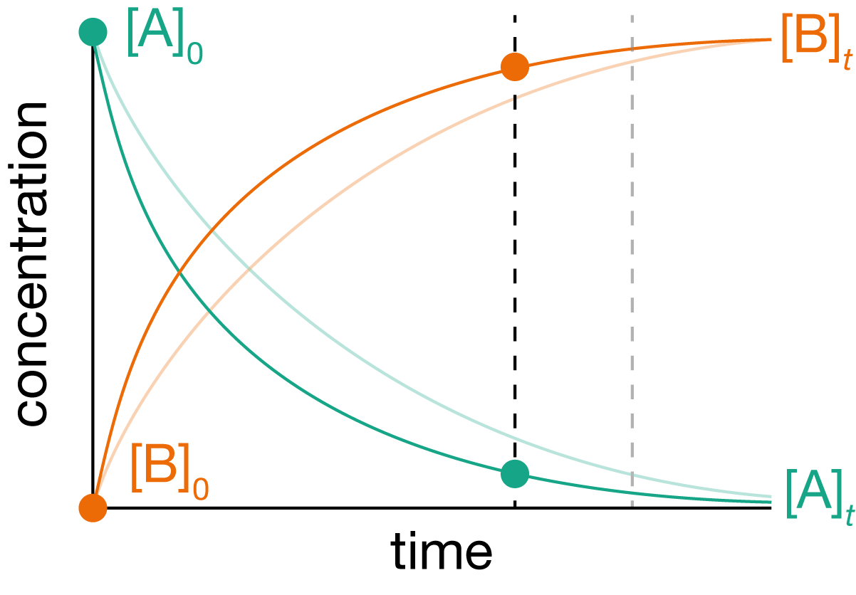
If we increase the temperature we (usually) expect our reaction to speed up. But by how much? If we increase the reaction temperature by 10 K, how much faster can we reach 90% yield?

Figure 1.2: If we increase the temperature we (usually) expect our reaction to speed up. But by how much? If we increase the reaction temperature by 10 K, how much faster can we reach 90% yield?

1.2 Reaction Rates

A core concept in chemical kinetics is the idea of a reaction rate — the speed at which chemical change happens. We express reaction rates mathematically as derivatives of the form $\frac{\mathrm{d}[\mathrm{X}]}{\mathrm{d}t}$, representing the change in concentration of a species X with time. This rate can be positive (for products being formed) or negative (for reactants being consumed).

For any reaction that does not have a 1:1 stoichiometry ratio between all reactants and products, the numerical “rate” will depend on the chemical species we choose to define this. For example, for the reaction

\[\begin{equation} \mathrm{A} \longrightarrow 2\mathrm{B} \end{equation}\]

the product, B, is formed at twice the rate that the reactant, A, is consumed. Hence,

\[2\frac{\mathrm{d}[\mathrm{A}]}{\mathrm{d}t} = \frac{\mathrm{d}[\mathrm{B}]}{\mathrm{d}t}\]

In general, we can define an “overall” reaction rate $\nu$ that is related to the rates of change of reactants and products by

\[\nu = \frac{1}{n_\mathrm{X}}\frac{\mathrm{d}[\mathrm{X}]}{\mathrm{d}t}\]

where $n_\mathrm{X}$ is the stoichiometric coefficient of species $X$ in the reaction equation.

1.3 Simple Rate Equations

For many reactions, the rate of reaction is proportional to the concentrations of the reactants, raised to some power; i.e.,

\[\nu = k [\mathrm{A}]^a [\mathrm{B}]^b [\mathrm{C}]^c \ldots\]

The proportionality constant, $k$, is called the rate constant. The exponents, $a$, $b$, $c$ …, describe the order of the reaction with respect to the reactants A, B, C ….

So, for a reaction

\[\mathrm{A} + \mathrm{B} \longrightarrow \mathrm{C}\]

with rate equation (or “rate law”)

\[\nu = k[\mathrm{A}]^2[\mathrm{B}]\],

we would describe this as being second-order with respect to A, and first-order with respect to B.

For rate equations that have the simple form above, we can define an overall order, which is the sum of the individual orders with respect to each of the reactants. In the example above, this reaction would be described as being third-order overall, since $a+b = 3$.

Not all reactions follow simple rate laws. For example, the reaction between H₂ and Br₂ to form HBr has an empirically-determined rate law

\[\begin{equation} \nu = k\frac{[\mathrm{H}_2][\mathrm{Br}_2]^\frac{1}{2}}{1+k^\prime [\mathrm{HBr}]/[\mathrm{Br}_2]} \tag{1.1} \end{equation}\]

This rate law is first-order with respect to H₂, because $\nu \propto [\mathrm{H_2}]$. But we cannot define an order with respect to Br₂, because the overall rate is not simply proportional to $[\mathrm{Br}_2]$ raised to some power. Instead, we would describe the order with respect to Br₂ as being undefined. This means the overall order is also undefined, since we cannot simply add the orders with respect to H₂ and Br₂.

1.4 Elementary Processes

Any chemical reaction can be broken down into a sequence of one of more single-step “elementary” processes.

For example, for the reaction $\mathrm{H}_2 + \mathrm{Br}_2 \longrightarrow 2\mathrm{HBr}$, where the empirical rate law is given by (1.1), one sequence of elementary processes that is consistent with this rate law is

\[\begin{eqnarray} \mathrm{Br}_2 & \longrightarrow & \mathrm{Br}^\bullet + \mathrm{Br}^\bullet \\ \mathrm{Br}^\bullet + \mathrm{H}_2 & \longrightarrow & \mathrm{H}^\bullet + \mathrm{HBr} \\ \mathrm{H}^\bullet + \mathrm{Br}_2 & \longrightarrow & \mathrm{Br}^\bullet + \mathrm{HBr} \\ \mathrm{Br}^\bullet + \mathrm{Br}^\bullet & \longrightarrow & \mathrm{Br}_2 \tag{1.2} \end{eqnarray}\]

1.4.1 Molecularity

Elementary processes can be classified according to their molecularity — the number of reactant molecules that must come together for a particular reaction step. For example, in reaction mechanism (1.2), the first step involves the dissociation of Br₂ to form two Br radicals:

\[\begin{equation} \mathrm{Br}_2 \longrightarrow \mathrm{Br}^\bullet + \mathrm{Br}^\bullet \end{equation}\]

This reaction step involves a single reactant molecule, so it is described a unimolecular.

The second step involves a Br radical and H₂ molecule reacting:

\[\begin{equation} \mathrm{Br}^\bullet + \mathrm{H}_2 \longrightarrow \mathrm{H}^\bullet + \mathrm{HBr} \end{equation}\]

Because two reactant molecules must come together for this step, this is described as a bimolecular process.

A process that involves two molecules of the same chemical species, as in the last step of the reaction mechanism above, is also bimolecular:

\[\begin{equation} \mathrm{Br}^\bullet + \mathrm{Br}^\bullet \longrightarrow \mathrm{Br}_2 \end{equation}\]

1.4.2 Rate Laws for Elementary Processes

The rate laws for elementary processes directly reflect their molecularity. Unimolecular processes ($\mathrm{A} \longrightarrow \mathrm{P}$) show first-order kinetics with rate $\nu = k[\mathrm{A}]$. Similarly, bimolecular processes show second-order kinetics: for a bimolecular process involving two distinct chemical species ($\mathrm{A} + \mathrm{B} \longrightarrow \mathrm{P}$), the process is first-order with respect to each species: $\nu = k[\mathrm{A}][\mathrm{B}]$, while a bimolecular process that involves two molecules of the same chemical species ($2\mathrm{A} \longrightarrow \mathrm{P}$) is second-order with respect to that species: $\nu = k[\mathrm{A}]^2$.

Termolecular processes, involving three reactant molecules, show third order kinetics, e.g., $\nu = k[\mathrm{A}]^2[\mathrm{B}]$. In general, termolecular processes are rare, because the probability of three molecules colliding simultaneously with the correct orientation is very small. While termolecular processes can play a role at very high pressure, under more typical reaction conditions, experimental observations of third-order kinetics are often better explained by a complex multistep reaction mechanism.

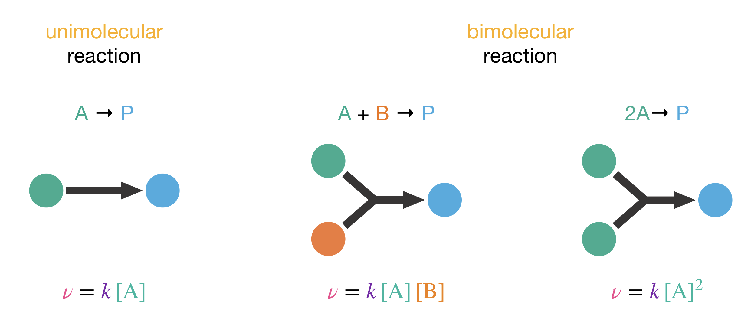
Elementary processes always follow simple rate laws, where the order with respect to each reactant reﬂects the molecularity of the process.

Figure 1.3: Elementary processes always follow simple rate laws, where the order with respect to each reactant reﬂects the molecularity of the process.

1.5 Moving Between Concentration and Rate Perspectives

The progression of any chemical reaction can be viewed from two complementary perspectives: the concentration of species as they change over time, $[\mathrm{A}]$, and the instantaneous rates at which these changes occur, $\mathrm{d}[\mathrm{A}]/\mathrm{d}t$. These two perspectives both describe the same underlying chemical process, just viewed through different mathematical lenses.

Consider a reactant A being consumed during a reaction. We might track its concentration $[\mathrm{A}]$ as it decreases over time, giving us a curve of concentration versus time. At any point on this curve, we can determine the instantaneous rate of reaction by finding the slope of the tangent line. Mathematically, this is equivalent to computing the derivative of $[\mathrm{A}]$, i.e., $\frac{\mathrm{d}[\mathrm{A}]}{\mathrm{d}t}$. Since we are dealing with the concentration of a reactant, the reaction rate is then the negative of this derivative (since the concentrations of A decreases with time):

\[\begin{equation} \nu = -\frac{\mathrm{d}[\mathrm{A}]}{\mathrm{d}t} \tag{1.3} \end{equation}\]

We can also go the other way from a description of rate to a description of the concentration profile over time. Mathematically we do this by integration, which is the inverse operation to differentiation. By integrating a rate, we effectively sum all the small changes in concentration over some time interval. For example, the change in concentration of A from the start of a reaction at $t=0$ is given by

\[\begin{equation} [\mathrm{A}]_t - [\mathrm{A}]_0 = \int_0^t -\nu(t)\,\mathrm{d}t \tag{1.4} \end{equation}\]

Whether we work in terms of concentrations or rates depends on the question we are trying to answer, what information we have available to us, and whether it is more mathematically convenient to work with one than the other.

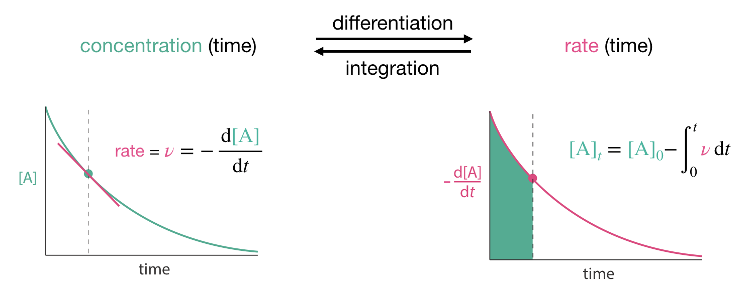
If we know the concentration of a reactant or product as a function of time we can calculate the rate of change of this concentration by differentiation. We can also calculate how concentrations vary in time from rates by the inverse procedure, integration.

Figure 1.4: If we know the concentration of a reactant or product as a function of time we can calculate the rate of change of this concentration by differentiation. We can also calculate how concentrations vary in time from rates by the inverse procedure, integration.

1.6 Integrating Simple Rate Laws

For simple rate laws of the form

\[\frac{\mathrm{d}[\mathrm{A}]}{\mathrm{d}t} = -k[\mathrm{A}]^n\]

we can derive corresponding integrated rate laws by integrating (see CH12002 Lecture 3).

1.6.1 First-Order Reactions

For a first-order process $\mathrm{A} \longrightarrow \mathrm{B}$, the rate of change of concentration of reactant, A, is given by

\[\begin{equation} \frac{\mathrm{d}[\mathrm{A}]}{\mathrm{d}t} = -k[\mathrm{A}] \end{equation}\]

To derive the corresponding integrated rate law, we rearrange this to form an integral equation:

\[\begin{equation} \int_{[\mathrm{A}]_0}^{\mathrm[A]_t} \frac{\mathrm{d}[\mathrm{A}]}{[\mathrm{A}]}\,\mathrm{d}[\mathrm{A}] = \int_0^t -k\,\mathrm{d}t \end{equation}\]

where the limits of the integral with respect to concentration of A are between the concentration at time $0$ ($[\mathrm{A}]_0$) and the concentration at time $t$ ($[\mathrm{A}]_t$), and the limits of the integral with respect to time are between $t=0$ and $t=t$.

Integrating, using the integral $\int \frac{1}{x}\,\mathrm{d}x = \ln x$, gives

\[\begin{equation} \ln [\mathrm{A}]_t - \ln [\mathrm{A}]_0 = -kt \end{equation}\]

which can be rearranged as

\[\begin{equation} [\mathrm{A}]_t = [\mathrm{A}]_0\mathrm{e}^{-kt} \tag{1.5} \end{equation}\]

Hence, for a first-order process, the concentration of the reactant decays exponentially with time.

Having derived an expression for $[\mathrm{A}]_t$ we can now derive the integrated rate law for the concentration of the product, B, as a function of time. To do so, we use the known stoichoimetry of the reaction: for every molecule of A consumed, one molecule of B is formed, so the total concentration $[\mathrm{A}] + [\mathrm{B}]$ must be constant. Furthermore, when $t=0$, only A is present, with a concentration $[\mathrm{A}]_0$. So, $[\mathrm{A}] + [\mathrm{B}] = [\mathrm{A}]_0$.

Substituting in our expression for $[\mathrm{A}]$ (Eqn. (1.5) gives

\[\begin{eqnarray} [\mathrm{B}] & = & [\mathrm{A}]_0 - [\mathrm{A}]_0\mathrm{e}^{-kt} \\ & = & [\mathrm{A}]_0\left(1-\mathrm{e}^{-kt}\right) \end{eqnarray}\]

Hence, for a first-order process, the concentration of the product exponentially approaches a limit of $[\mathrm{B}]_t = [\mathrm{A}]_0$.

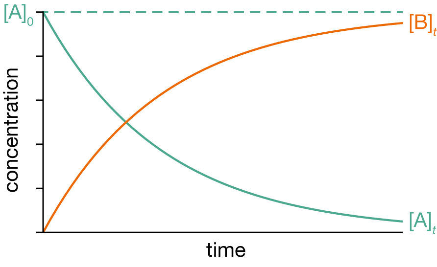
$Concentrations as a function of time for a first-order process $\mathrm{A} \longrightarrow \mathrm{B}$.$

Figure 1.5: Concentrations as a function of time for a first-order process $\mathrm{A} \longrightarrow \mathrm{B}$.

1.6.2 Second-Order Reactions

For a second-order process $2\mathrm{A} \longrightarrow \mathrm{B}$, with overall rate $\nu = \frac{\mathrm{d}[\mathrm{B}]}{\mathrm{d}t}$, the rate of change of concentration of reactant, A, is

\[\begin{equation} \frac{\mathrm{d}[\mathrm{A}]}{\mathrm{d}t} = -2k[\mathrm{A}]^2 \tag{1.6} \end{equation}\]

As for first-order reactions, above, we can derive the corresponding integrated rate law for $[\mathrm{A}]_t$ by rearranging Eqn. (1.6) and then integrating:

\[\begin{equation} \int_{[\mathrm{A}]_0}^{\mathrm[A]_t} \frac{\mathrm{d}[\mathrm{A}]}{[\mathrm{A}]^2}\,\mathrm{d}[\mathrm{A}] = \int_0^t -k\,\mathrm{d}t \end{equation}\]

Integrating, using the integral $\int \frac{1}{x^2}\,\mathrm{d}x = -\frac{1}{x}$, gives

\[\begin{equation} \frac{1}{[\mathrm{A}]_t} - \frac{1}{[\mathrm{A}]_0} = -kt \end{equation}\]

which can be rearranged as

\[\begin{equation} [\mathrm{A}]_t = \frac{[\mathrm{A}]_0}{1 + kt[\mathrm{A}]_0} \end{equation}\]

To obtain an expression for $[\mathrm{B}]_t$, we again use our knowledge of the reaction stoichiometry and initial conditions: we start with only the reactant A, and at any stage of the reaction, the amount of B formed is equal to half the amount of A consumed.

\[\begin{equation} [\mathrm{B}]_t = \frac{1}{2}\left([\mathrm{A}]_0 - [\mathrm{A}]_t\right) \end{equation}\]

And, so

\[\begin{equation} [\mathrm{B}]_t = \frac{[\mathrm{A}]_0}{2}\left(1 - \frac{1}{1+kt[\mathrm{A}_0]}\right) \end{equation}\]

which rearranges to

\[\begin{equation} [\mathrm{B}]_t = \frac{kt[\mathrm{A}]_0^2}{2(1 + kt[\mathrm{A}]_0)} \end{equation}\]

$Concentrations as a function of time for a second-order process $2\mathrm{A} \longrightarrow \mathrm{B}$. The dashed line shows the sum $[\mathrm{A}]_t + [\mathrm{B}]_t$.$

Figure 1.6: Concentrations as a function of time for a second-order process $2\mathrm{A} \longrightarrow \mathrm{B}$. The dashed line shows the sum $[\mathrm{A}]_t + [\mathrm{B}]_t$.

Aside: Why Does Our Second-Order Rate Equation Include a Factor of 2?

Let us briefly examine the origin of the factor of 2 on the right-hand side of Eqn. @ref{eq:secondorderdiff}. Writing the rate equation for $\frac{\mathrm{d}[\mathrm{A}]}{\mathrm{d}t}$ in this way is consistent with the convention in Section 1.2, that the overall rate of a reaction is related to the rates of change of specific reactants or products by

\[\begin{equation} \nu = \frac{1}{n_\mathrm{X}}\frac{\mathrm{d}[\mathrm{X}]}{\mathrm{d}t} \tag{1.7} \end{equation}\]

We can also justify the factor of $2$ by recognising that the stoichiometry of the reaction requires 2 molecules of A to be consumed for every 1 molecule of B formed, and, hence,

\[\begin{equation} \frac{\mathrm{d}[\mathrm{A}]}{\mathrm{d}t} = 2\frac{\mathrm{d}[\mathrm{B}]}{\mathrm{d}t} \end{equation}\]

The factor of 2 in Eqn. (1.6) is somewhat arbitrary though, as it is a consequence of our choice to define the overall rate of reaction as $\nu = \frac{\mathrm{d}[\mathrm{B}]}{\mathrm{d}t}$. If, instead, we define our overall rate as $\nu = \frac{\mathrm{d}[\mathrm{A}]}{\mathrm{d}t}$ then we would write the rate of change of concentration of A as

\[\begin{equation} \frac{\mathrm{d}[\mathrm{A}]}{\mathrm{d}t} = -k[\mathrm{A}]^2 \tag{1.8} \end{equation}\]

The functional form for $\frac{\mathrm{d}[\mathrm{A}]}{\mathrm{d}t}$ is the same in both cases (Eqns. (1.6) and (1.8). Our choice of how we define our overall rate, however, determines what the rate constant $k$ actually describes. The rate constant in (1.8) is equal to twice the rate constant in (1.6). Upon reflection, it should perhaps not be surprising that the numerical value of our rate constant $k$ depends on how we choose to define the reaction rate. Whichever of these two ways we choose to define our overall rate, the procedure for deriving the second-order intergrated rate law is unchanged, and we end up with the same functional form for the integrated rate law — either with, or without, the factor of 2 carried through the derivation.

1.7 From Mechanisms to Rate Laws

The relationship between reaction mechanisms and the time evolution of chemical concentrations depends strongly on the complexity of the reaction scheme. For reactions that consist of a single elementary process, we can usually determine how the concentrations of reactants and products evolve with time through a straightforward two-step process:

Write down the rate equations for reactants and products based on the molecularity of the elementary process
Directly integrate these rate equations to obtain the corresponding integrated rate laws

For example, we have already seen how this works for first-order processes in Section 1.6. For reactions with multistep mechanisms, however, the path from mechanism to time evolution is often more complex. Our starting point is always the reaction mechanism itself—the sequence of elementary processes that describes the complete reaction scheme. From this mechanism, we write differential rate equations for all chemical species that appear, including not only the reactants and products, but also any reaction intermediates. When analysing multistep mechanisms, we typically pursue one or both of two goals:

To derive an expression for the overall reaction rate in terms of reactant concentrations only, eliminating any dependence on intermediate concentrations To obtain integrated rate laws that describe how the concentrations of reactants and products vary with time

How we approach these goals depends on the nature of the reaction mechanism under consideration. In general, we can analyse complex reaction mechanisms using one of three strategies:

1.7.1 Exact Solutions

For some reaction mechanisms, we can derive exact analytical solutions to our coupled differential rate equations. While this approach is the most mathematically satisfying, it is only possible for relatively simple reaction schemes.

1.7.2 Approximate Analytical Solutions

More commonly, we can simplify our set of coupled differential equations by applying chemical approximations based on the physical nature of the reaction mechanism. We then solve these simplified equations to obtain analytical solutions that accurately describe the real system within the range of conditions where our approximations hold. This approach often provides valuable chemical insight into the factors controlling reaction rates and time evolution.

1.7.3 Numerical Integration

When analytical solutions prove intractable, we can always fall back on numerical methods. By numerically integrating our differential rate equations, we can model how the concentrations of all species—reactants, products, and intermediates—evolve over time. While this approach will always work in principle, it may provide less direct insight into the underlying chemical processes than analytical solutions, even approximate ones. Although numerical integration provides a reliable method of last resort, there is often significant value in pursuing analytical solutions, either exact or approximate. These solutions can reveal fundamental relationships between reaction parameters and chemical behavior that might be obscured in purely numerical results.

1.8 Consecutive Reactions

Having examined simple rate laws and elementary processes, we now consider how to analyze reactions that occur in multiple steps. One important class of such reactions are consecutive (or sequential) reactions, where products are formed through a series of steps:

\[\mathrm{A} \xrightarrow{k_1} \mathrm{B} \xrightarrow{k_2} \mathrm{C}\]

Such reaction sequences are common in both chemical and biochemical systems. For example, the decomposition of many organic compounds proceeds through multiple intermediates, and many metabolic pathways involve sequences of enzyme-catalyzed reactions.

1.8.1 Rate Equations

Following our approach from Section 1.2, we can write differential rate equations for each species:

\[\begin{align} \frac{\mathrm{d}[\mathrm{A}]}{\mathrm{d}t} &= -k_1[\mathrm{A}] \\ \frac{\mathrm{d}[\mathrm{B}]}{\mathrm{d}t} &= +k_1[\mathrm{A}] - k_2[\mathrm{B}] \\ \frac{\mathrm{d}[\mathrm{C}]}{\mathrm{d}t} &= +k_2[\mathrm{B}] \end{align}\]

Note that species B appears both as a product (in the first step) and as a reactant (in the second step). This is characteristic of reaction intermediates.

1.8.2 Integrated Rate Laws

We can solve these coupled differential equations sequentially. First, the equation for [A] is a simple first-order decay (see Section 1.6):

\[[\mathrm{A}] = [\mathrm{A}]_0\mathrm{e}^{-k_1t}\]

To solve for [B], we substitute this expression into the second differential equation:

\[\frac{\mathrm{d}[\mathrm{B}]}{\mathrm{d}t} = k_1[\mathrm{A}]_0\mathrm{e}^{-k_1t} - k_2[\mathrm{B}]\]

Integrating this linear first-order differential equation (see Appendix A) gives:

\[[\mathrm{B}] = \frac{k_1[\mathrm{A}]_0}{k_2-k_1}(\mathrm{e}^{-k_1t} - \mathrm{e}^{-k_2t})\]

Finally, we can find [C] using conservation of mass ([A] + [B] + [C] = [A]₀):

\[[\mathrm{C}] = [\mathrm{A}]_0\left[1 + \frac{k_1\mathrm{e}^{-k_2t} - k_2\mathrm{e}^{-k_1t}}{k_1-k_2}\right]\]

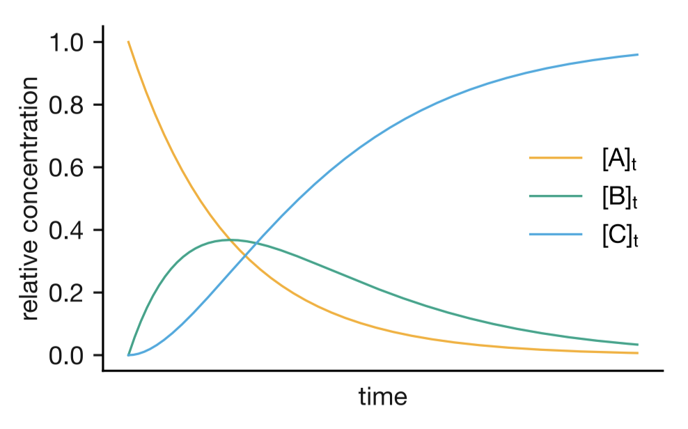
Figure 1.7: Concentration profiles for a consecutive reaction A → B → C. The intermediate B exhibits a maximum concentration at intermediate times.

1.8.3 Limiting Cases and the Rate-Determining Step

The kinetics of consecutive reactions can be simplified when one step is much slower than the other. This slower step becomes rate-determining for the overall reaction.

1.8.3.1 Case 1: $k_1 \ll k_2$

When the first step is much slower than the second:

B is consumed almost as soon as it is formed
[B] remains very small throughout the reaction
Formation of C follows approximately first-order kinetics:

\[[\mathrm{C}] \approx [\mathrm{A}]_0(1-\mathrm{e}^{-k_1t})\]

1.8.3.2 Case 2: $k_1 \gg k_2$

When the first step is much faster than the second:

A is rapidly converted to B
B accumulates before slowly converting to C
After an initial rapid phase, formation of C follows approximately first-order kinetics:

\[[\mathrm{C}] \approx [\mathrm{A}]_0(1-\mathrm{e}^{-k_2t})\]

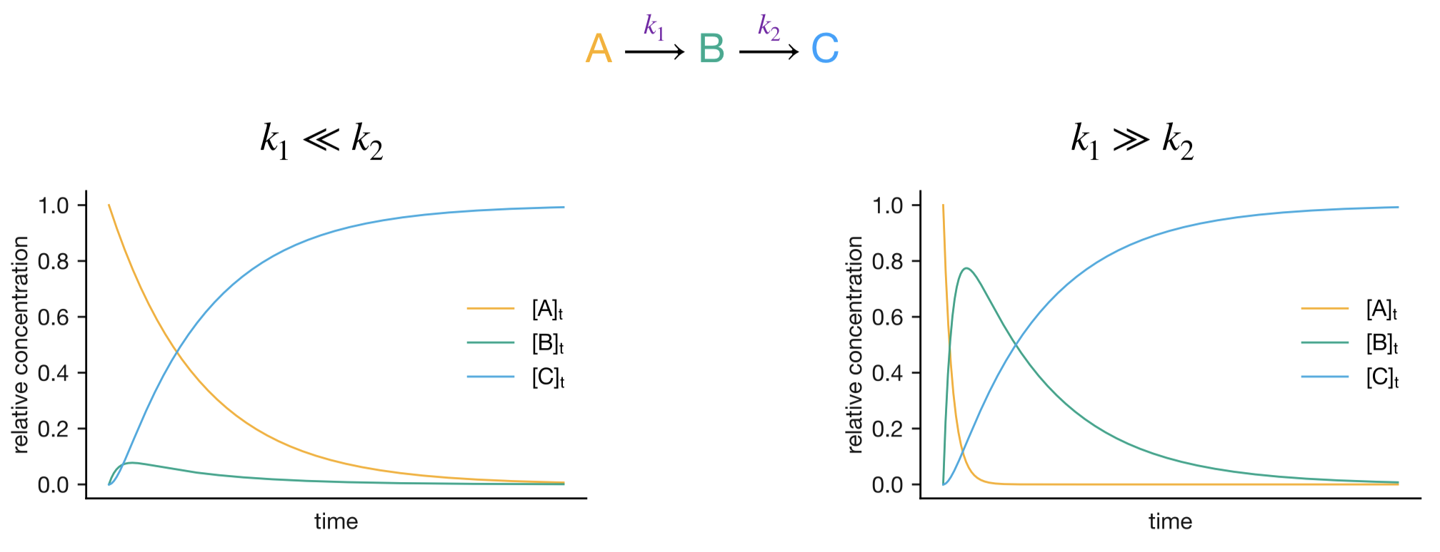
Concentration profiles for consecutive reactions in limiting cases. Left: k₁ << k₂, where the first step is rate-determining. Right: k₁ >> k₂, where the second step is rate-determining.

Figure 1.8: Concentration profiles for consecutive reactions in limiting cases. Left: k₁ << k₂, where the first step is rate-determining. Right: k₁ >> k₂, where the second step is rate-determining.

The concept of a rate-determining step is particularly valuable when analyzing complex reaction mechanisms. When one step in a reaction sequence is much slower than the others, it becomes the “bottleneck” that controls the overall reaction rate. This principle helps explain why many complex reactions show simple kinetic behavior—the observed kinetics often reflect just the rate-determining step.

1.9 The Steady-State Approximation

When analyzing complex reaction mechanisms, we can often simplify our analysis using the steady-state approximation. This approximation applies to reaction intermediates that are consumed much faster than they are formed, leading to a “steady state” where the rate of change of the intermediate’s concentration is approximately zero.

1.9.1 Basic Principles

The steady-state approximation assumes that after a brief initial period, the concentration of a reactive intermediate B reaches a “steady state” where:

\[\frac{\mathrm{d}[\mathrm{B}]}{\mathrm{d}t} \approx 0\]

Consider our consecutive reaction mechanism from the previous section:

\[\mathrm{A} \xrightarrow{k_1} \mathrm{B} \xrightarrow{k_2} \mathrm{C}\]

The rate equations are:

\[\begin{align} \frac{\mathrm{d}[\mathrm{A}]}{\mathrm{d}t} &= -k_1[\mathrm{A}] \\ \frac{\mathrm{d}[\mathrm{B}]}{\mathrm{d}t} &= k_1[\mathrm{A}] - k_2[\mathrm{B}] \\ \frac{\mathrm{d}[\mathrm{C}]}{\mathrm{d}t} &= k_2[\mathrm{B}] \end{align}\]

When $k_2 \gg k_1$, B is consumed much faster than it is formed, and we can apply the steady-state approximation:

\[\frac{\mathrm{d}[\mathrm{B}]}{\mathrm{d}t} = k_1[\mathrm{A}] - k_2[\mathrm{B}] \approx 0\]

This allows us to solve for $[\mathrm{B}]$:

\[[\mathrm{B}] \approx \frac{k_1}{k_2}[\mathrm{A}]\]

Substituting this expression into our rate equation for C:

\[\frac{\mathrm{d}[\mathrm{C}]}{\mathrm{d}t} = k_2[\mathrm{B}] = k_1[\mathrm{A}]\]

From conservation of mass, $[\mathrm{A}]_0 = [\mathrm{A}] + [\mathrm{B}] + [\mathrm{C}]$. Under the condition $k_2 \gg k_1$, the concentration of B remains small, so $[\mathrm{A}]_0 ≈ [\mathrm{A}] + [\mathrm{C}]$. Therefore:

\[\frac{\mathrm{d}[\mathrm{C}]}{\mathrm{d}t} = k_1[\mathrm{A}] = k_1([A]_0 - [C])\]

This first-order differential equation can be directly integrated to give:

\[[\mathrm{C}] = [\mathrm{A}]_0(1-\mathrm{e}^{-k_1t})\]

This is the same result we obtained in our analysis of consecutive reactions in the limit where $k_1 \ll k_2$.

1.9.2 Validity of the Steady-State Approximation

The steady-state approximation simplifies the analysis of complex reaction mechanisms by treating the concentrations of reactive intermediates as constant. While this mathematical convenience makes many problems tractable, we need to understand when the approximation holds and what it reveals about reaction kinetics.

A steady state exists when the rates of formation and consumption of the intermediate balance. This requires two conditions: the intermediate must be consumed much faster than it forms, and enough time must have passed for the intermediate to build up to its steady-state concentration. This initial period, where the intermediate concentration increases to its steady-state value, is called the induction period.

Consider a reaction with the mechanism:

\[\mathrm{A} + \mathrm{B} \underset{k_{-1}}{\overset{k1}\rightleftharpoons} \mathrm{C} \overset{k_2}\rightarrow \mathrm{D}\]

Reactants A and B combine reversibly to form an intermediate C, which then reacts to form product D. The steady-state approximation assumes $\mathrm{d}[\mathrm{C}]/\mathrm{d}t \approx 0$ — that is, the concentration of C remains approximately constant as the reaction proceeds.

$Time evolution of concentrations for the reaction mechanism $\mathrm{A} + \mathrm{B} \underset{k_1}{\overset{k1}\rightleftharpoons} \mathrm{C} \overset{k_2}\longrightarrow \mathrm{D}$ where $k_2 \gg k_1$. Solid lines show the exact concentrations, while the dashed line shows the predicted product concentration $[\mathrm{D}]_\mathrm{SSA}$ calculated using the steady-state approximation for intermediate C. The approximation overshoots during the initial induction period where [C] is still building up, but describes the reaction progress well once steady state is established.$

Figure 1.9: Time evolution of concentrations for the reaction mechanism $\mathrm{A} + \mathrm{B} \underset{k_1}{\overset{k1}\rightleftharpoons} \mathrm{C} \overset{k_2}\longrightarrow \mathrm{D}$ where $k_2 \gg k_1$. Solid lines show the exact concentrations, while the dashed line shows the predicted product concentration $[\mathrm{D}]_\mathrm{SSA}$ calculated using the steady-state approximation for intermediate C. The approximation overshoots during the initial induction period where [C] is still building up, but describes the reaction progress well once steady state is established.

Figure 1.9 compares the steady-state prediction for [D] (dashed line) with the exact concentration profiles (solid lines) when $k_2 \gg k_1$. During the induction period, the steady-state approximation overestimates the rate of product formation because it assumes C has already reached its steady-state concentration. However, once this period passes, the predicted and actual concentrations align well.

These observations suggest several criteria for applying the steady-state approximation to new systems. First, the kinetics must support the basic steady-state assumption, typically requiring $k_2 \gg k_1$. Second, the timescale of interest must exceed the induction period. Third, any deviations during the induction period should not compromise the analysis.

When steady-state predictions match experimental data, they provide evidence for a reaction mechanism involving an intermediate maintained at near-constant concentration during the main reaction phase.

CH22008 Lecture Notes