Lecture 11 Temperature Effects on Reaction Rates

We have spent this course treating rate constants as fixed numbers: we measure $k$, use it to predict how concentrations evolve, and extract mechanistic information from how $k$ depends on concentration. But we have not asked what determines the value of $k$ itself. A full answer to that question is beyond the scope of this course, but one piece of the puzzle is accessible: rate constants depend on temperature, and this dependence encodes information about energy barriers and reaction mechanisms that concentration data alone cannot provide.

11.1 The Arrhenius Equation

Rate constants for most reactions increase with temperature. We refrigerate food to slow the chemical reactions that cause it to spoil; we heat reaction mixtures to make sluggish reactions proceed at a practical rate. But how exactly does $k$ depend on $T$? Figure 11.1 shows a typical example: the relationship is not linear, with $k$ rising slowly at low temperatures and much more steeply at high temperatures.

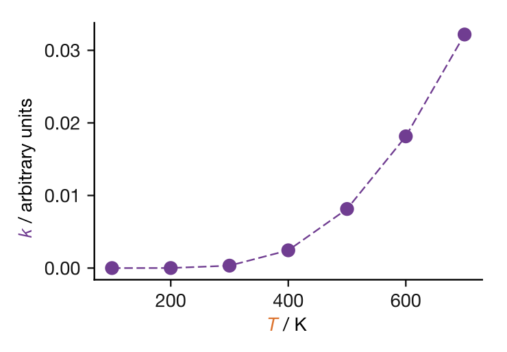
Rate constant $k$ plotted against temperature for a typical reaction. The relationship is not linear: $k$ increases slowly at low temperatures and much more steeply at high temperatures.

Figure 11.1: Rate constant $k$ plotted against temperature for a typical reaction. The relationship is not linear: $k$ increases slowly at low temperatures and much more steeply at high temperatures.

In 1889, Svante Arrhenius examined published rate data for several reactions and found that they were all reasonably well described by a single expression, which we now call the Arrhenius equation:

\[\begin{equation} k = A\,\mathrm{e}^{-E_\mathrm{a}/RT} \tag{11.1} \end{equation}\]

where $R$ is the gas constant. The two parameters, $A$ and $E_\mathrm{a}$, are called the pre-exponential factor and activation energy respectively. These are empirical parameters, obtained by fitting to experimental measurements. The equation says that $k$ increases exponentially with temperature, with the steepness of that increase governed by $E_\mathrm{a}$.

Taking the natural logarithm of both sides converts the Arrhenius equation into a linear form:

\[\begin{equation} \ln k = \ln A - \frac{E_\mathrm{a}}{R} \cdot \frac{1}{T} \tag{11.2} \end{equation}\]

This has the form $y = c + mx$ with $y = \ln k$ and $x = 1/T$. A plot of $\ln k$ versus $1/T$ is called an Arrhenius plot.

11.2 Extracting Arrhenius Parameters from Data

The most reliable way to extract $A$ and $E_\mathrm{a}$ from experimental data is to fit the Arrhenius equation (Eqn. (11.1)) directly by nonlinear regression — this is straightforward with modern computational tools. Historically, however, the standard approach has been to use the linearised form (Eqn. (11.2)): plot $\ln k$ against $1/T$, fit a straight line, and read off $E_\mathrm{a}$ from the slope ($-E_\mathrm{a}/R$) and $A$ from the intercept ($\ln A$). This is still the method presented in many textbooks, and it has the practical advantage of being tractable with pen and paper — including under exam conditions. If the data are well described by the Arrhenius equation, the Arrhenius plot gives a straight line (Figure 11.2). A steeper slope corresponds to a larger $E_\mathrm{a}$: the rate constant is more sensitive to temperature.

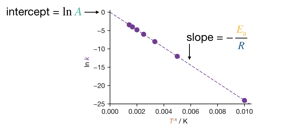
$Arrhenius plot ($\ln k$ versus $1/T$) for two reactions with different activation energies. The slope of each line is $-E_\mathrm{a}/R$, so a steeper line corresponds to a larger activation energy and a stronger temperature dependence.$

Figure 11.2: Arrhenius plot ($\ln k$ versus $1/T$) for two reactions with different activation energies. The slope of each line is $-E_\mathrm{a}/R$, so a steeper line corresponds to a larger activation energy and a stronger temperature dependence.

When data are available at only two temperatures, we can estimate $E_\mathrm{a}$ directly. Writing Eqn. (11.2) at temperatures $T_1$ and $T_2$ and subtracting to eliminate $\ln A$ gives:

\[\begin{equation} \ln\frac{k_2}{k_1} = \frac{E_\mathrm{a}}{R}\left(\frac{1}{T_1} - \frac{1}{T_2}\right) \tag{11.3} \end{equation}\]

This is useful in both directions: given $k$ at two temperatures we can find $E_\mathrm{a}$, and given $E_\mathrm{a}$ and $k$ at one temperature we can predict $k$ at another.

You should be able to: Use the Arrhenius equation to construct an Arrhenius plot and extract $E_\mathrm{a}$ and $A$, and apply the two-temperature formula (Eqn. (11.3)) to calculate $E_\mathrm{a}$ from rate constants at two temperatures or to predict a rate constant at a new temperature.

11.3 What Do $E_\mathrm{a}$ and $A$ Tell Us?

So far, $A$ and $E_\mathrm{a}$ are just numbers we extract from a fit. For elementary reactions, however, they have concrete physical meanings.

Consider the simplest possible atom-transfer reaction: H + H–H $\rightarrow$ H–H + H. Reactants and products are identical, so the overall energy change is zero. But the reaction cannot happen instantaneously. As the incoming H atom approaches, the existing H–H bond must stretch and weaken while the new bond begins to form. At the midpoint, the central hydrogen is partially bonded to both neighbours in a symmetric [H$\cdots$H$\cdots$H] configuration. Two partial bonds cost more energy than one full bond, so this configuration is higher in energy than either the reactants or the products.

The energy difference between this highest-energy configuration and the reactants is the energy barrier for the reaction. The progress from reactants through the top of the barrier to products is described by a reaction coordinate, and the energy along this coordinate gives the energy profile shown in Figure 11.3.

$Energy profile for the symmetric reaction H + H$_2$ $\rightarrow$ H$_2$ + H. Reactants and products are at the same energy. At the top of the barrier, neither bond is fully formed.$

Figure 11.3: Energy profile for the symmetric reaction H + H$_2$ $\rightarrow$ H$_2$ + H. Reactants and products are at the same energy. At the top of the barrier, neither bond is fully formed.

For many elementary reactions, the system must pass through a high-energy configuration on the way from reactants to products. The energy profile along the reaction coordinate then has a maximum, and the height of that maximum above the reactants is the energy barrier for the reaction. When reactants and products have different energies, the energy profile is asymmetric and the forward and reverse barriers differ: for an exothermic reaction, the forward barrier is lower than the reverse barrier (Figure 11.4).

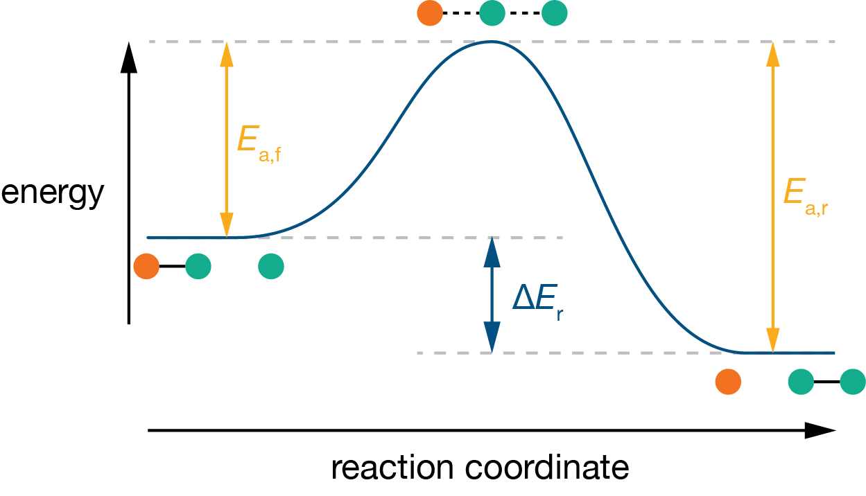
$Energy profile for an asymmetric reaction. The products are lower in energy than the reactants, so the forward activation energy $E_\mathrm{a,f}$ is smaller than the reverse activation energy $E_\mathrm{a,r}$. The difference between the two barriers equals the overall energy change $\Delta E$.$

Figure 11.4: Energy profile for an asymmetric reaction. The products are lower in energy than the reactants, so the forward activation energy $E_\mathrm{a,f}$ is smaller than the reverse activation energy $E_\mathrm{a,r}$. The difference between the two barriers equals the overall energy change $\Delta E$.

We now have a microscopic picture (elementary reactions have energy barriers) and a macroscopic fitting parameter $E_\mathrm{a}$ from the Arrhenius equation. What connects the two?

At any temperature, molecules have a spread of energies. In thermal equilibrium, the fraction of molecules with energy exceeding some threshold $E$ is approximately proportional to $\mathrm{e}^{-E/RT}$ — this is the Boltzmann distribution.² Figure 11.5 illustrates this for the relative kinetic energy in bimolecular collisions: only collisions to the right of the threshold line have enough energy to surmount the barrier, and this fraction grows substantially at higher temperature.

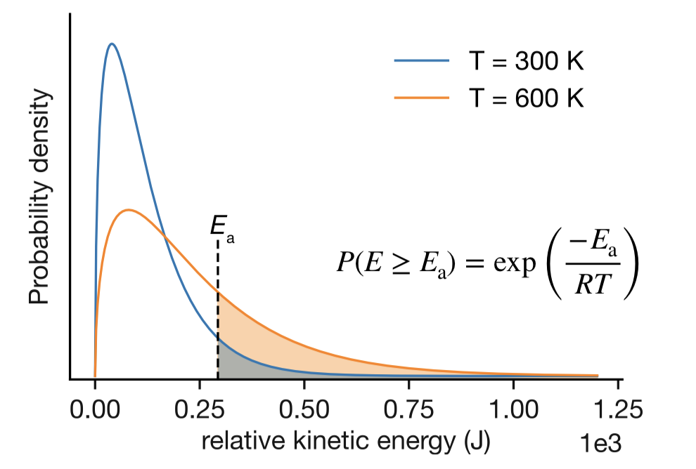
$Distribution of relative kinetic energies in molecular collisions at two temperatures, $T_1$ and $T_2 > T_1$. The shaded regions show the fraction of collisions with energy exceeding the threshold $E_\mathrm{a}$. This fraction is approximately proportional to $\mathrm{e}^{-E_\mathrm{a}/RT}$.$

Figure 11.5: Distribution of relative kinetic energies in molecular collisions at two temperatures, $T_1$ and $T_2 > T_1$. The shaded regions show the fraction of collisions with energy exceeding the threshold $E_\mathrm{a}$. This fraction is approximately proportional to $\mathrm{e}^{-E_\mathrm{a}/RT}$.

If a reaction requires molecules to exceed an energy barrier $E$, and the fraction doing so goes as $\mathrm{e}^{-E/RT}$, then the rate constant should contain this factor — and the barrier height should appear as $E_\mathrm{a}$ in the Arrhenius equation. This is the physical connection: for an elementary reaction, the empirical $E_\mathrm{a}$ obtained from an Arrhenius fit corresponds to the height of the energy barrier that molecules must overcome to react. The argument is illustrated here for kinetic energy in bimolecular collisions, but the exponential dependence on energy is a general feature of thermal equilibrium, applying equally to vibrational energy in unimolecular reactions or energy along a reaction coordinate. The exponential sensitivity of reaction rates to temperature arises because only a small fraction of molecules have enough energy to cross the barrier.

The remaining factors that determine the rate constant are collected into the pre-exponential factor $A$. For a bimolecular elementary step, $A$ reflects how often molecules encounter each other in a suitable orientation. For a unimolecular step, $A$ reflects how often energy accumulates in the vibrational mode that leads to reaction. In both cases, $A$ plays the role of an attempt frequency — how often molecules are in a position to cross the barrier — while the exponential factor gives the fraction of those attempts that succeed.

11.4 Reading an Arrhenius Plot: The Sign of $E_\mathrm{a}$

We now know what $E_\mathrm{a}$ represents for an elementary reaction. What can its value tell us about mechanism? If the data on an Arrhenius plot fall on a straight line, the slope is $-E_\mathrm{a}/R$. The sign of the slope (and therefore the sign of $E_\mathrm{a}$) carries mechanistic information.

Most reactions have rate constants that increase with temperature, giving a negative slope on the Arrhenius plot and a positive $E_\mathrm{a}$. For an elementary step, this reflects a genuine energy barrier. For a multi-step mechanism, $E_\mathrm{a}$ is still positive but does not correspond to a single barrier: it is an empirical composite of the activation energies of the individual elementary steps. These two cases are indistinguishable from the Arrhenius plot alone; mechanistic information is needed to interpret the number.

Some reactions show very weak temperature dependence, with $E_\mathrm{a} \approx 0$ and a nearly flat Arrhenius plot. Radical–radical recombinations are an example: two radicals combining to form a bond does not require either partner to partially break an existing bond first (contrast with the bond-rearrangement argument above), so the energy barrier is negligible. The rate is limited by how often the radicals encounter each other, not by the energy of those encounters.

The Boltzmann argument from the previous section tells us why $k$ increases with $T$ for any process with a barrier: a higher temperature puts more molecules above the threshold energy. Occasionally, however, a rate constant decreases with increasing temperature, giving a positive slope on the Arrhenius plot and a negative apparent $E_\mathrm{a}$ (Figure 11.6).

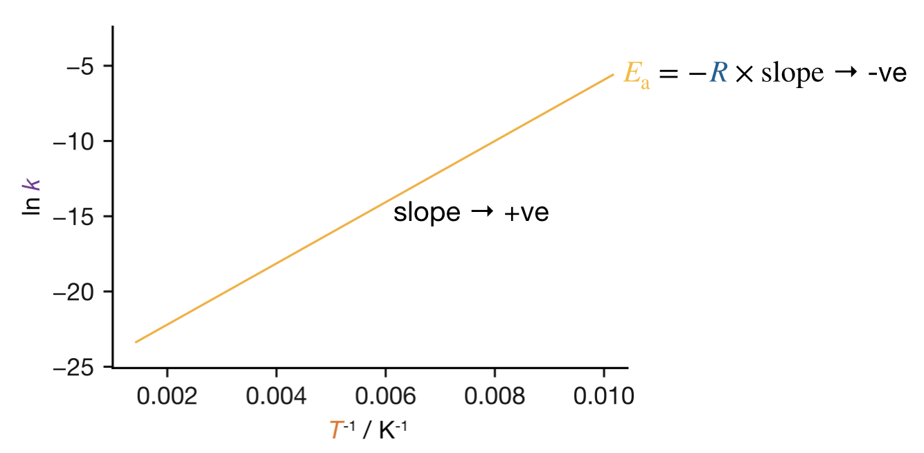
Arrhenius plot for a reaction with a negative apparent activation energy. The positive slope indicates that the rate constant decreases with increasing temperature.

Figure 11.6: Arrhenius plot for a reaction with a negative apparent activation energy. The positive slope indicates that the rate constant decreases with increasing temperature.

A single elementary step cannot have a negative $E_\mathrm{a}$. The energy barrier for an elementary step is either positive (when the system must pass through a high-energy configuration) or zero (when no rearrangement is required), but it cannot be negative. All elementary activation energies are therefore $\geq 0$, and a negative apparent $E_\mathrm{a}$ is direct evidence for a multi-step mechanism.

The oxidation of NO provides a well-studied example. In Lecture 7 we analysed the pre-equilibrium mechanism for this reaction and found $k_\mathrm{obs} = k_2 K$, where $K$ is the equilibrium constant for the dimerisation NO + NO $\rightleftharpoons$ (NO)₂. As temperature increases, $k_2$ increases (it is an elementary step with a barrier), but $K$ decreases: two separate NO molecules have far more translational freedom than a single (NO)₂ dimer, so the dissociated state has higher entropy, and increasing temperature favours it. The decrease in $K$ more than offsets the increase in $k_2$, and the net effect is that $k_\mathrm{obs}$ decreases with temperature.

You should be able to: Explain why the NO oxidation reaction has a negative apparent activation energy, and why negative apparent $E_\mathrm{a}$ implies a multi-step mechanism.

11.5 When the Arrhenius Plot Is Not Linear

The Arrhenius equation predicts a straight line on the Arrhenius plot. This prediction rests on the assumption that $A$ and $E_\mathrm{a}$ are constants, independent of temperature. For many reactions this is a good approximation, but real data sometimes show curvature, telling us that $E_\mathrm{a}$ is itself varying with temperature. We can accommodate this with a more general definition of the activation energy as the local slope of the Arrhenius plot:

\[\begin{equation} E_\mathrm{a}(T) = -R\frac{\mathrm{d}(\ln k)}{\mathrm{d}(1/T)} \tag{11.4} \end{equation}\]

This is the local slope of the Arrhenius plot at each temperature, multiplied by $-R$. When the plot is linear, $E_\mathrm{a}(T)$ is constant and equal to the Arrhenius $E_\mathrm{a}$. The Arrhenius equation is the special case of Eqn. (11.4) where the activation energy does not depend on temperature.

A common cause of curvature is competing pathways. When two parallel reactions contribute to the observed rate, $k_\mathrm{obs} = k_1 + k_2$, and each pathway has its own Arrhenius parameters. At low temperatures, the pathway with the lower $E_\mathrm{a}$ dominates because its exponential factor $\mathrm{e}^{-E_\mathrm{a}/RT}$ decreases less steeply with $1/T$. At high temperatures, both exponential factors approach unity and the larger pre-exponential factor wins: if the higher-$E_\mathrm{a}$ pathway also has the larger $A$, it takes over.³ The Arrhenius plot shows two approximately linear regions with different slopes, connected by a curve (Figure 11.7).

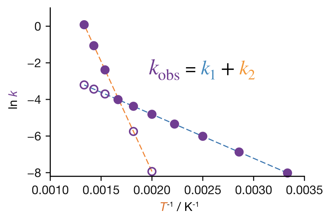
$Arrhenius plot for a reaction with two competing pathways. Dashed lines show the individual rate constants $k_1$ (low $E_\mathrm{a}$, low $A$) and $k_2$ (high $E_\mathrm{a}$, high $A$). The solid curve shows $k_\mathrm{obs} = k_1 + k_2$. At low temperatures the low-$E_\mathrm{a}$ pathway dominates; at high temperatures the high-$E_\mathrm{a}$ pathway takes over.$

Figure 11.7: Arrhenius plot for a reaction with two competing pathways. Dashed lines show the individual rate constants $k_1$ (low $E_\mathrm{a}$, low $A$) and $k_2$ (high $E_\mathrm{a}$, high $A$). The solid curve shows $k_\mathrm{obs} = k_1 + k_2$. At low temperatures the low-$E_\mathrm{a}$ pathway dominates; at high temperatures the high-$E_\mathrm{a}$ pathway takes over.

Temperature data therefore complement the concentration data we have worked with throughout this course. Concentration measurements give us the rate law, which constrains the mechanism; temperature measurements reveal energy barriers and test mechanistic proposals. In Lecture 1 we asked how temperature affects reaction rates. The Arrhenius equation describes this dependence; the Boltzmann factor makes the exponential form physically plausible; and the details of the Arrhenius plot (its slope, its sign, and its curvature) encode information about the energy landscape and the mechanism of the reaction.

Key Concepts

The Arrhenius equation, $k = A\,\mathrm{e}^{-E_\mathrm{a}/RT}$, is an empirical model that describes how rate constants depend on temperature. The parameters $A$ and $E_\mathrm{a}$ are obtained by fitting to experimental data.
An Arrhenius plot ($\ln k$ vs $1/T$) gives a straight line with slope $-E_\mathrm{a}/R$ and intercept $\ln A$ when the Arrhenius equation holds. The two-temperature formula allows $E_\mathrm{a}$ to be determined from measurements at two temperatures, or $k$ to be predicted at a new temperature.
For a single elementary step, $E_\mathrm{a}$ corresponds to the height of the energy barrier along the reaction coordinate, and $A$ reflects the rate at which molecules attempt to cross it.
The exponential temperature dependence is consistent with the Boltzmann factor: the fraction of molecules with energy exceeding a threshold goes approximately as $\mathrm{e}^{-E_\mathrm{a}/RT}$.
A negative apparent $E_\mathrm{a}$ is impossible for a single elementary step and therefore implies a multi-step mechanism.
For multi-step mechanisms, the measured $E_\mathrm{a}$ is a composite that does not correspond to a single microscopic barrier.
A curved Arrhenius plot indicates that $E_\mathrm{a}$ varies with temperature. The general definition $E_\mathrm{a}(T) = -R\,\mathrm{d}(\ln k)/\mathrm{d}(1/T)$ gives the local activation energy, which reduces to the constant Arrhenius $E_\mathrm{a}$ when the plot is linear.
Temperature dependence complements concentration dependence as a probe of reaction mechanisms.

In the Boltzmann distribution, the probability of a molecule occupying a microstate with energy $E$ is proportional to $\mathrm{e}^{-E/k_\mathrm{B}T}$, where $k_\mathrm{B}$ is the Boltzmann constant ($R = N_\mathrm{A}k_\mathrm{B}$). When several microstates share the same energy, the probability of having that energy is $g\,\mathrm{e}^{-E/k_\mathrm{B}T}$, where $g$ is the degeneracy. The fraction of molecules exceeding a threshold energy is dominated by the exponential factor.↩︎
If the higher-$E_\mathrm{a}$ pathway does not also have the larger $A$, the lower-$E_\mathrm{a}$ pathway dominates at all temperatures and no crossover occurs.↩︎

CH12002 Lecture Notes

Lecture 11 Temperature Effects on Reaction Rates

11.1 The Arrhenius Equation

11.2 Extracting Arrhenius Parameters from Data

11.3 What Do \(E_\mathrm{a}\) and \(A\) Tell Us?

11.4 Reading an Arrhenius Plot: The Sign of \(E_\mathrm{a}\)

11.5 When the Arrhenius Plot Is Not Linear

Key Concepts