Lecture 2 Integrated Rate Laws

In the previous chapter, we saw that rate laws provide a window into how reactions work at the molecular level. The formation of HI has the simple rate law $\nu = k[\mathrm{H}_2][\mathrm{I}_2]$, but the formation of HBr (despite its similar stoichiometry) follows a complex rate law that reflects a multi-step chain mechanism. Different mechanisms produce different rate laws. To use rate laws as a tool for understanding mechanisms, however, we first need to be able to extract them from experimental data.

The challenge is that our rate laws are written in terms of rates, derivatives such as $\mathrm{d}[\mathrm{A}]/\mathrm{d}t$, whereas what we typically measure in the laboratory is concentration as a function of time. Consider, for example, the thermal decomposition of azomethane (CH₃N₂CH₃), studied at $2.18 \times 10^4\,\mathrm{Pa}$ and $576\,\mathrm{K}$:

$t$ / min	0	30	60	90	120	150	180
$[\text{azomethane}]$ / $10^{-3}\,\mathrm{mol\,dm}^{-3}$	8.70	6.52	4.89	3.67	2.75	2.06	1.55

What is the rate law for this reaction? What is the rate constant? We cannot answer these questions just by inspecting the raw data. We need a strategy for connecting our differential rate laws to concentration–time measurements.

The approach is straightforward: propose a rate law, integrate it to predict how $[\mathrm{A}]_t$ should depend on time, and then compare that prediction with the experimental data. If the prediction fits, we have our rate law and rate constant; if not, we try a different order.

2.1 Zeroth-Order Reactions

To integrate a differential rate law, we use the technique of separation of variables: we rearrange so that everything involving concentration is on one side and everything involving time is on the other, then integrate each side independently between appropriate limits (using the techniques from the Mathematical Foundations chapter). This gives us the integrated rate law: an equation that tells us the concentration $[\mathrm{A}]_t$ as a function of time. We then rearrange this into a linear form suitable for graphical analysis.

For a zeroth-order reaction, the rate is constant, independent of the concentration of the reactant:

\[\frac{\mathrm{d}[\mathrm{A}]}{\mathrm{d}t} = -k\]

The variables are already separated (concentration on the left, time on the right), so we integrate both sides between $t = 0$ (when $[\mathrm{A}] = [\mathrm{A}]_0$) and time $t$ (when $[\mathrm{A}] = [\mathrm{A}]_t$):

\[\int_{[\mathrm{A}]_0}^{[\mathrm{A}]_t} \mathrm{d}[\mathrm{A}] = \int_0^t -k\,\mathrm{d}t\]

\[[\mathrm{A}]_t - [\mathrm{A}]_0 = -kt\]

Rearranging gives the zeroth-order integrated rate law:

\[\begin{equation} [\mathrm{A}]_t = [\mathrm{A}]_0 - kt \tag{2.1} \end{equation}\]

The differential rate law and this integrated form are two equivalent descriptions of zeroth-order kinetics: one tells us the instantaneous rate of change, the other the accumulated change from the start of the reaction.

Eqn. (2.1) is already in linear form: a plot of $[\mathrm{A}]_t$ against $t$ gives a straight line with slope $-k$ and intercept $[\mathrm{A}]_0$ (Figure 2.1). Physically, a constant rate means the reaction proceeds at the same speed regardless of how much reactant remains, a situation that can arise, for example, when a reaction is limited by a saturated catalyst surface.

$Zeroth-order kinetics: $[\mathrm{A}]$ decreases linearly with time. A plot of $[\mathrm{A}]$ versus $t$ gives a straight line with slope $-k$ and intercept $[\mathrm{A}]_0$. The concentration reaches zero at $t = [\mathrm{A}]_0/k$, after which the model no longer applies.$

Figure 2.1: Zeroth-order kinetics: $[\mathrm{A}]$ decreases linearly with time. A plot of $[\mathrm{A}]$ versus $t$ gives a straight line with slope $-k$ and intercept $[\mathrm{A}]_0$. The concentration reaches zero at $t = [\mathrm{A}]_0/k$, after which the model no longer applies.

2.2 First-Order Reactions

For a first-order reaction, the rate is proportional to the concentration of the reactant:

\[\frac{\mathrm{d}[\mathrm{A}]}{\mathrm{d}t} = -k[\mathrm{A}]\]

We separate variables and integrate:

\[\frac{\mathrm{d}[\mathrm{A}]}{[\mathrm{A}]} = -k\,\mathrm{d}t\]

\[\int_{[\mathrm{A}]_0}^{[\mathrm{A}]_t} \frac{\mathrm{d}[\mathrm{A}]}{[\mathrm{A}]} = \int_0^t -k\,\mathrm{d}t\]

\[\ln[\mathrm{A}]_t - \ln[\mathrm{A}]_0 = -kt\]

This gives the first-order integrated rate law in linear form:

\[\begin{equation} \ln[\mathrm{A}]_t = \ln[\mathrm{A}]_0 - kt \tag{2.2} \end{equation}\]

A plot of $\ln[\mathrm{A}]_t$ against $t$ gives a straight line with slope $-k$ and intercept $\ln[\mathrm{A}]_0$ (Figure 2.2). Taking the exponential of both sides gives the equivalent exponential form:

\[\begin{equation} [\mathrm{A}]_t = [\mathrm{A}]_0\,\mathrm{e}^{-kt} \tag{2.3} \end{equation}\]

This is the exponential decay we derived from general principles in the Mathematical Foundations chapter: whenever a quantity changes at a rate proportional to its current value, the result is an exponential function. First-order kinetics means the concentration decreases by the same fraction in each successive time interval. If 25% decomposes in the first 30 minutes, then 25% of what remains decomposes in the next 30 minutes, and the next, regardless of how much is left.

$First-order kinetics: $[\mathrm{A}]$ decays exponentially, so a plot of $\ln[\mathrm{A}]$ versus $t$ gives a straight line with slope $-k$ and intercept $\ln[\mathrm{A}]_0$. The concentration approaches zero asymptotically but never reaches it.$

Figure 2.2: First-order kinetics: $[\mathrm{A}]$ decays exponentially, so a plot of $\ln[\mathrm{A}]$ versus $t$ gives a straight line with slope $-k$ and intercept $\ln[\mathrm{A}]_0$. The concentration approaches zero asymptotically but never reaches it.

2.3 Second-Order Reactions

For a reaction that is second order in a single reactant:

\[\frac{\mathrm{d}[\mathrm{A}]}{\mathrm{d}t} = -k[\mathrm{A}]^2\]

Separating variables and integrating:

\[\frac{\mathrm{d}[\mathrm{A}]}{[\mathrm{A}]^2} = -k\,\mathrm{d}t\]

\[\int_{[\mathrm{A}]_0}^{[\mathrm{A}]_t} \frac{\mathrm{d}[\mathrm{A}]}{[\mathrm{A}]^2} = \int_0^t -k\,\mathrm{d}t\]

\[-\frac{1}{[\mathrm{A}]_t} + \frac{1}{[\mathrm{A}]_0} = -kt\]

Rearranging:

\[\begin{equation} \frac{1}{[\mathrm{A}]_t} = \frac{1}{[\mathrm{A}]_0} + kt \tag{2.4} \end{equation}\]

A plot of $1/[\mathrm{A}]_t$ against $t$ gives a straight line with slope $+k$ and intercept $1/[\mathrm{A}]_0$ (Figure 2.3). Notice that the slope is positive here, unlike the zeroth- and first-order cases where it is negative. Physically, because the rate depends on the square of the concentration, halving the concentration quarters the rate. Second-order reactions therefore slow down much more dramatically than first-order reactions as the reactant is consumed.

$Second-order kinetics: $[\mathrm{A}]$ decays more slowly than exponentially as the rate drops with the square of the concentration. A plot of $1/[\mathrm{A}]$ versus $t$ gives a straight line with slope $+k$ (positive, unlike the zeroth- and first-order cases) and intercept $1/[\mathrm{A}]_0$.$

Figure 2.3: Second-order kinetics: $[\mathrm{A}]$ decays more slowly than exponentially as the rate drops with the square of the concentration. A plot of $1/[\mathrm{A}]$ versus $t$ gives a straight line with slope $+k$ (positive, unlike the zeroth- and first-order cases) and intercept $1/[\mathrm{A}]_0$.

Aside: The Factor of 2 in Second-Order Rate Laws

Some textbooks write the second-order integrated rate law with an extra factor of 2 in front of $k$. This arises when the reaction is an elementary process, $2\mathrm{A} \rightarrow \text{products}$, and we account for the stoichiometric factor from Chapter 1. Each reaction event consumes two molecules of A, so $\mathrm{d}[\mathrm{A}]/\mathrm{d}t = -2k[\mathrm{A}]^2$, and the factor of 2 carries through the integration to give $1/[\mathrm{A}]_t = 1/[\mathrm{A}]_0 + 2kt$. Whether the 2 appears explicitly or is absorbed into the definition of $k$ is a matter of convention (it does not change the underlying chemistry), but it can cause confusion when comparing results from different sources. In these notes we use $k$ to absorb any stoichiometric factors, consistent with the convention in Chapter 1.

You should be able to: Derive the integrated rate law for a zeroth-, first-, or second-order reaction starting from the differential rate law, using separation of variables and integration.

2.4 Distinguishing Reaction Orders by Graphical Analysis

Each reaction order produces a different linear relationship, making it possible to distinguish them by plotting the same data in three different ways. The table below collects the key results, and Figure 2.4 shows the corresponding concentration profiles and linear plots.

Order	Integrated form	Linear plot	Slope
0	$[\mathrm{A}]_t = [\mathrm{A}]_0 - kt$	$[\mathrm{A}]$ vs $t$	$-k$
1	$[\mathrm{A}]_t = [\mathrm{A}]_0\,\mathrm{e}^{-kt}$	$\ln[\mathrm{A}]$ vs $t$	$-k$
2	$\frac{1}{[\mathrm{A}]_t} = \frac{1}{[\mathrm{A}]_0} + kt$	$\frac{1}{[\mathrm{A}]}$ vs $t$	$+k$

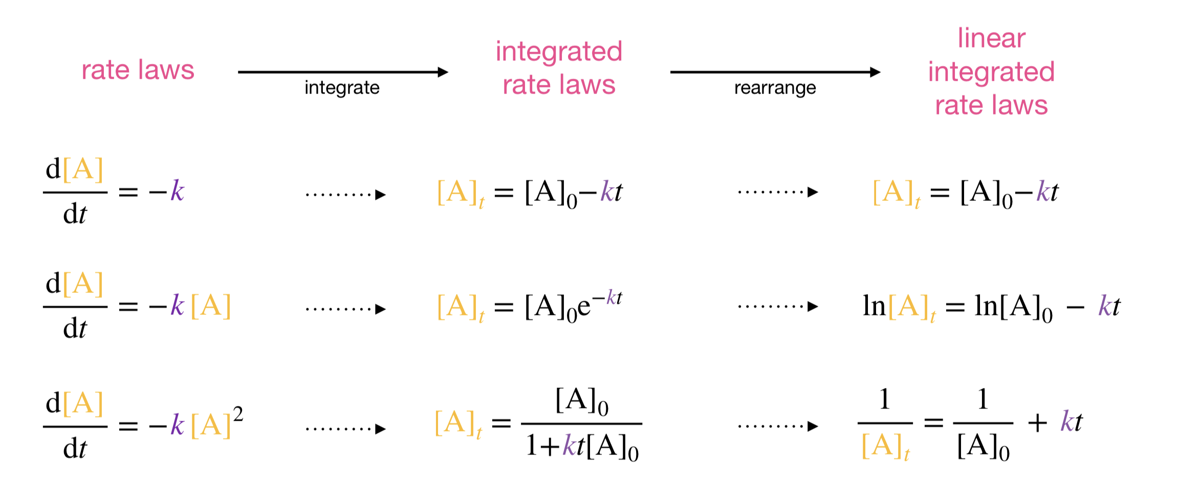
Concentration--time profiles (left) and the corresponding linear plots (right) for zeroth-, first-, and second-order reactions. Each reaction order produces a distinct curve shape, but differences are much easier to identify in the linear plots: data that obey a given rate law fall on a straight line, while data that do not show systematic curvature.

Figure 2.4: Concentration–time profiles (left) and the corresponding linear plots (right) for zeroth-, first-, and second-order reactions. Each reaction order produces a distinct curve shape, but differences are much easier to identify in the linear plots: data that obey a given rate law fall on a straight line, while data that do not show systematic curvature.

Each reaction order predicts a different functional form for concentration as a function of time—a different curve shape. We could, in principle, plot the raw concentration–time data and try to judge whether the curve looks exponential (first-order), linear (zeroth-order), or like $1/(a + bt)$ (second-order). In practice, though, judging whether a curve matches one functional form rather than another is very difficult by eye, and even simple statistical tests work much better with linear data. By rearranging each integrated rate law into a linear form, we turn the problem into one where the answer is much easier to see: data that are consistent with a particular rate law will fall on a straight line in the corresponding plot, while data that are inconsistent will show systematic curvature.

We can therefore test candidate rate laws by plotting the same dataset in each of the three linear forms and seeing which (if any) gives a straight line. The slope of that line gives the rate constant.

These graphical tests apply whenever a reaction follows a simple rate law of the form $\nu = k[\mathrm{A}]^n$ (including non-integer orders such as $n = \tfrac{1}{2}$), regardless of whether the underlying mechanism involves a single step or multiple steps. This is an important distinction: graphical analysis tells us the rate law, not the mechanism. A reaction that gives a straight line on a first-order plot might be a simple unimolecular decomposition, or it might involve a complex sequence of steps that happens to produce an overall first-order rate law. Determining the rate law is the essential first step; working out the mechanism requires further investigation.

2.5 Worked Example: Decomposition of Azomethane

Which of our three models fits the azomethane data from the start of this chapter? We test each of the three integrated rate laws by plotting the data in the corresponding linear form. Figure 2.5 shows the result: plotting $\ln[\text{azomethane}]$ against $t$ gives a straight line, consistent with first-order kinetics, with slope $-k = -9.6 \times 10^{-3}\,\mathrm{min}^{-1}$. The other two linear forms—$[\text{azomethane}]$ against $t$ and $1/[\text{azomethane}]$ against $t$—show clear curvature, ruling out zeroth- and second-order rate laws.

$Testing the azomethane decomposition data against each linear form. Only the first-order plot ($\ln[\text{azomethane}]$ vs $t$, centre) gives a straight line; the zeroth-order (left) and second-order (right) plots show systematic curvature. The slope of the first-order plot gives $k = 9.6 \times 10^{-3}\,\mathrm{min}^{-1}$.$

Figure 2.5: Testing the azomethane decomposition data against each linear form. Only the first-order plot ($\ln[\text{azomethane}]$ vs $t$, centre) gives a straight line; the zeroth-order (left) and second-order (right) plots show systematic curvature. The slope of the first-order plot gives $k = 9.6 \times 10^{-3}\,\mathrm{min}^{-1}$.

We now have our answer to the question posed at the start of this chapter: the decomposition of azomethane follows first-order kinetics, with a rate constant of $k = 9.6 \times 10^{-3}\,\mathrm{min}^{-1}$.

You should be able to: Test whether concentration–time data are consistent with a given reaction order by plotting in the appropriate linear form, and extract the rate constant from the slope.

2.6 Reactions with Two Different Reactants

The integrated rate laws above all involve a single reactant species. For a reaction between two different species, $\mathrm{A} + \mathrm{B} \rightarrow \text{products}$, the differential rate law is:

\[\frac{\mathrm{d}[\mathrm{A}]}{\mathrm{d}t} = -k[\mathrm{A}][\mathrm{B}]\]

Integration is more complex here because the right-hand side contains two concentrations that both change with time. The problem can be solved analytically using mass balance and partial fractions, giving the full integrated result:

\[\begin{equation} kt = \frac{1}{[\mathrm{B}]_0 - [\mathrm{A}]_0} \ln\!\left(\frac{[\mathrm{B}]_t / [\mathrm{B}]_0}{[\mathrm{A}]_t / [\mathrm{A}]_0}\right) \tag{2.5} \end{equation}\]

The derivation of this result is given in Appendix A; you are not expected to reproduce it. The result requires $[\mathrm{A}]_0 \neq [\mathrm{B}]_0$, since otherwise the denominator is zero. If the initial concentrations are equal, the problem reduces to the single-reactant second-order case (Eqn. (2.4)).

A common simplification, the isolation method, is to use one reactant in large excess. If $[\mathrm{B}]_0$ is, say, 100 times larger than $[\mathrm{A}]_0$, then even after all of A has reacted, $[\mathrm{B}]$ has decreased by only 1%. For practical purposes $[\mathrm{B}]$ remains constant throughout the reaction, and the rate law simplifies to:

\[\frac{\mathrm{d}[\mathrm{A}]}{\mathrm{d}t} \approx -k'[\mathrm{A}] \quad \text{where } k' = k[\mathrm{B}]_0\]

This is called a pseudo-first-order rate law: the reaction is second-order overall, but behaves as first-order under these conditions. The problem reduces to the first-order integrated rate law we have already derived, and all of the graphical analysis from this chapter applies directly.

2.7 Key Concepts

The rate law tells us about the reaction mechanism, so extracting rate laws from experimental data is a central goal of chemical kinetics.
Integrated rate laws relate concentration to time, connecting differential rate laws to experimentally measurable quantities.
The strategy is: propose a rate law, integrate to predict $[\mathrm{A}]_t$, and compare with data.
Each reaction order gives a different integrated rate law with a characteristic linear form.
Plotting data in the appropriate linear form tests whether a given rate law is consistent with the data. A straight line is consistent with the proposed order; the slope gives the rate constant.
For zeroth-order: $[\mathrm{A}]$ vs $t$ is linear (slope $-k$). For first-order: $\ln[\mathrm{A}]$ vs $t$ is linear (slope $-k$). For second-order: $1/[\mathrm{A}]$ vs $t$ is linear (slope $+k$).
First-order kinetics corresponds to exponential decay: $[\mathrm{A}]_t = [\mathrm{A}]_0\,\mathrm{e}^{-kt}$.
Reactions between two different species can be simplified to pseudo-first-order kinetics by using one reactant in large excess.

Order	Integrated form	Linear plot	Slope
0	\([\mathrm{A}]_t = [\mathrm{A}]_0 - kt\)	\([\mathrm{A}]\) vs \(t\)	\(-k\)
1	\([\mathrm{A}]_t = [\mathrm{A}]_0\,\mathrm{e}^{-kt}\)	\(\ln[\mathrm{A}]\) vs \(t\)	\(-k\)
2	\(\frac{1}{[\mathrm{A}]_t} = \frac{1}{[\mathrm{A}]_0} + kt\)	\(\frac{1}{[\mathrm{A}]}\) vs \(t\)	\(+k\)