Lecture 1 Introduction to Chemical Kinetics
1.1 Why Study Reaction Kinetics?
Chemistry is fundamentally concerned with change: the transformation of substances into new forms with different properties. When we mix reactants together, we want to know not just whether a reaction will occur, but how rapidly it will proceed. While thermodynamics provides powerful tools for determining whether a particular chemical change is favourable and what the final equilibrium composition will be, it cannot tell us how quickly this equilibrium will be reached.
A reaction may be thermodynamically favourable yet proceed so slowly that it appears not to happen at all. Consider the conversion of diamond to graphite: this is thermodynamically spontaneous at room temperature and pressure, yet the process occurs at such a negligible rate that diamonds are stable over geological timescales. Conversely, some reactions reach equilibrium in fractions of a second.
Chemical kinetics tells us how fast a reaction proceeds. But kinetics reveals more than just speed: because different molecular-level mechanisms lead to different rate laws, measuring how fast a reaction occurs can tell us how it occurs.
1.2 Describing How Concentrations Change with Time
Let us examine a simple reaction: the conversion of a reactant A into a product B:
\[\mathrm{A} \rightarrow \mathrm{B}\]
We track the progress of this reaction by monitoring concentrations as functions of time. Using square brackets to denote concentration (in \(\mathrm{mol\,dm}^{-3}\)), we write these time-dependent concentrations as \([\mathrm{A}]_t\) and \([\mathrm{B}]_t\). As the reaction proceeds, A is consumed and its concentration falls, while B is formed and its concentration rises, as illustrated in Figure 1.1.
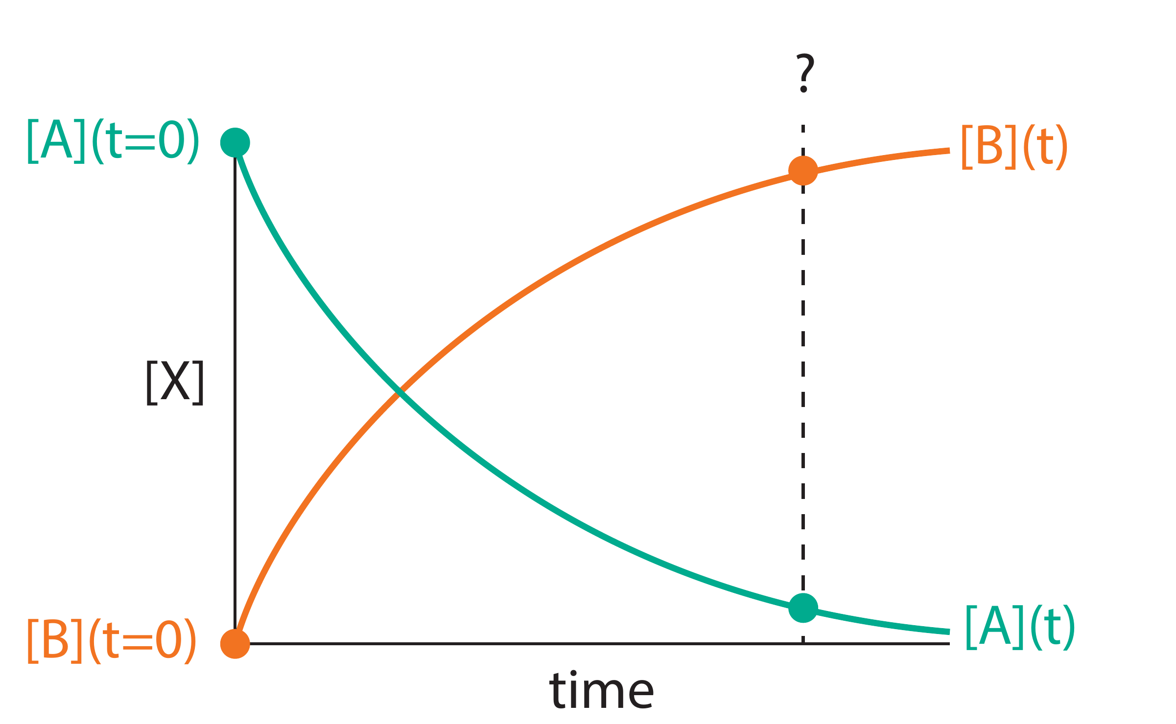
Figure 1.1: Time evolution of concentrations for the reaction A → B. As the reaction proceeds, the concentration of reactant A decreases while the concentration of product B increases. At any time \(t\), the sum of the two concentrations equals the initial concentration of A (assuming we start with pure A).
Starting from initial values at \(t = 0\), the system evolves toward its final state. We might ask how much product B is present after a given time, how long it takes for a certain percentage of A to convert, or how changes in temperature or concentration affect the reaction speed. Answering these questions requires us to understand how reaction rates relate to concentrations.
1.3 Reaction Rates
We quantify how quickly a reaction occurs in terms of the rate at which concentrations change with time. For our simple A → B reaction, the reaction rate can be expressed as either the rate of disappearance of A or the rate of appearance of B. If the rate were constant, calculating it would be straightforward: we would simply measure the change in concentration over a time interval:
\[\text{change in [A] per unit time} = \frac{[\mathrm{A}]_{t_2} - [\mathrm{A}]_{t_1}}{t_2 - t_1} = \frac{\Delta[\mathrm{A}]}{\Delta t}\]
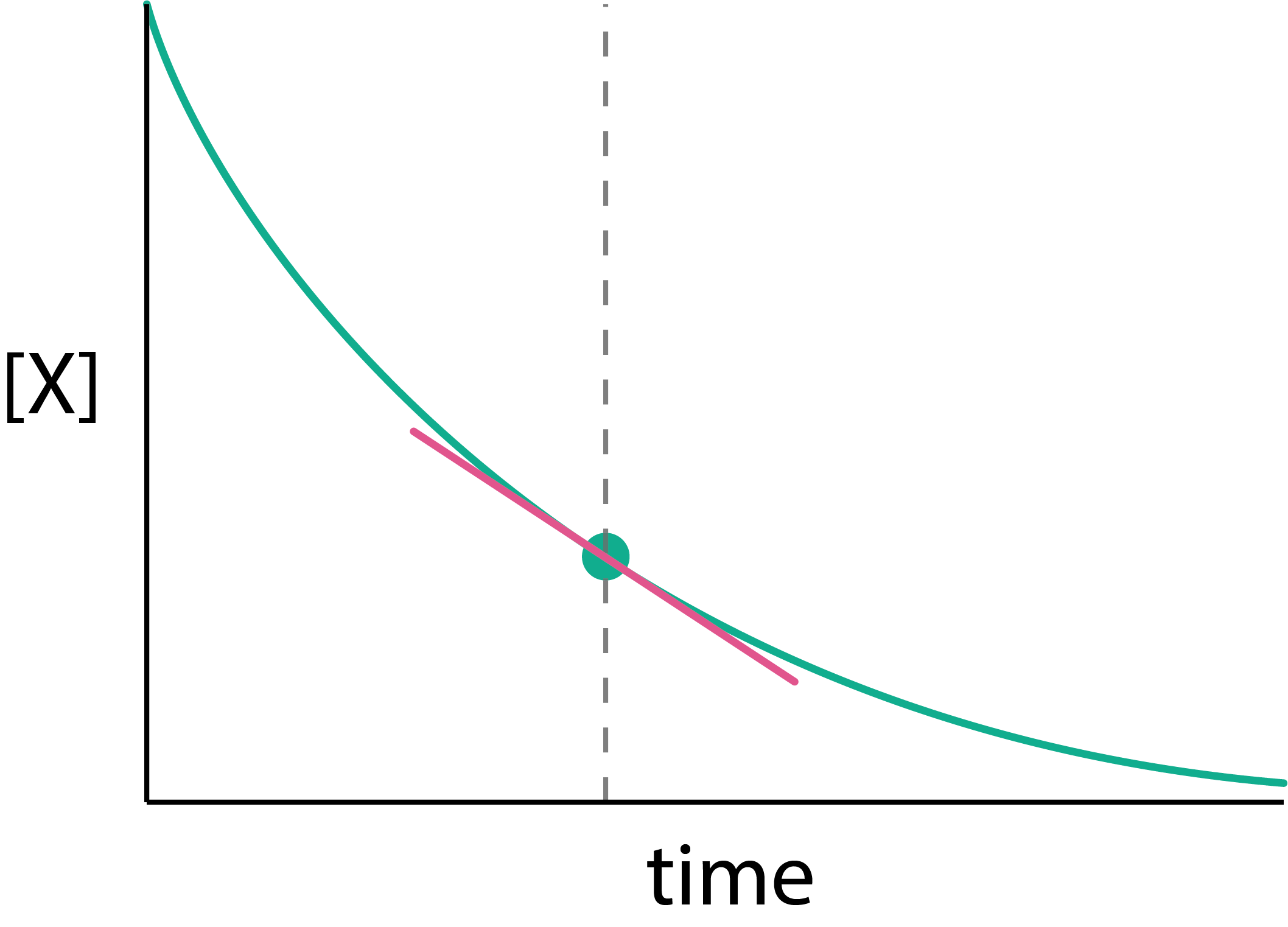
Figure 1.2: The reaction rate at any instant equals the slope of the tangent to the concentration-time curve at that point. For a reaction where the rate decreases over time (as reactant is consumed), the slope becomes less steep as the reaction progresses.
In general, however, reaction rates are not constant; reactions typically slow down as reactant is consumed. The ratio \(\Delta[\mathrm{A}]/\Delta t\) gives only the average rate over the interval \(\Delta t\). To describe the rate at a particular instant, we take the limit as \(\Delta t \rightarrow 0\). Geometrically, this means drawing a tangent to the concentration–time curve at the time of interest; the slope of that tangent is the instantaneous rate (Figure 1.2). Formally, this limit defines the derivative, and we can write the rate in terms of either species:
\[\text{rate} = -\frac{\mathrm{d}[\mathrm{A}]}{\mathrm{d}t} = +\frac{\mathrm{d}[\mathrm{B}]}{\mathrm{d}t}\]
Because \([\mathrm{A}]\) decreases with time, \(\mathrm{d}[\mathrm{A}]/\mathrm{d}t\) is negative. The minus sign in the first expression ensures the rate comes out positive, consistent with the convention that reaction rates are always positive quantities. The units of reaction rate are concentration per unit time: \(\mathrm{mol\,dm}^{-3}\,\mathrm{s}^{-1}\).
For reactions with more complex stoichiometry, the relationship between concentration changes requires appropriate stoichiometric factors. Consider a reaction where one molecule of A combines with two molecules of B to form one molecule of C:
\[\mathrm{A} + 2\mathrm{B} \rightarrow \mathrm{C}\]
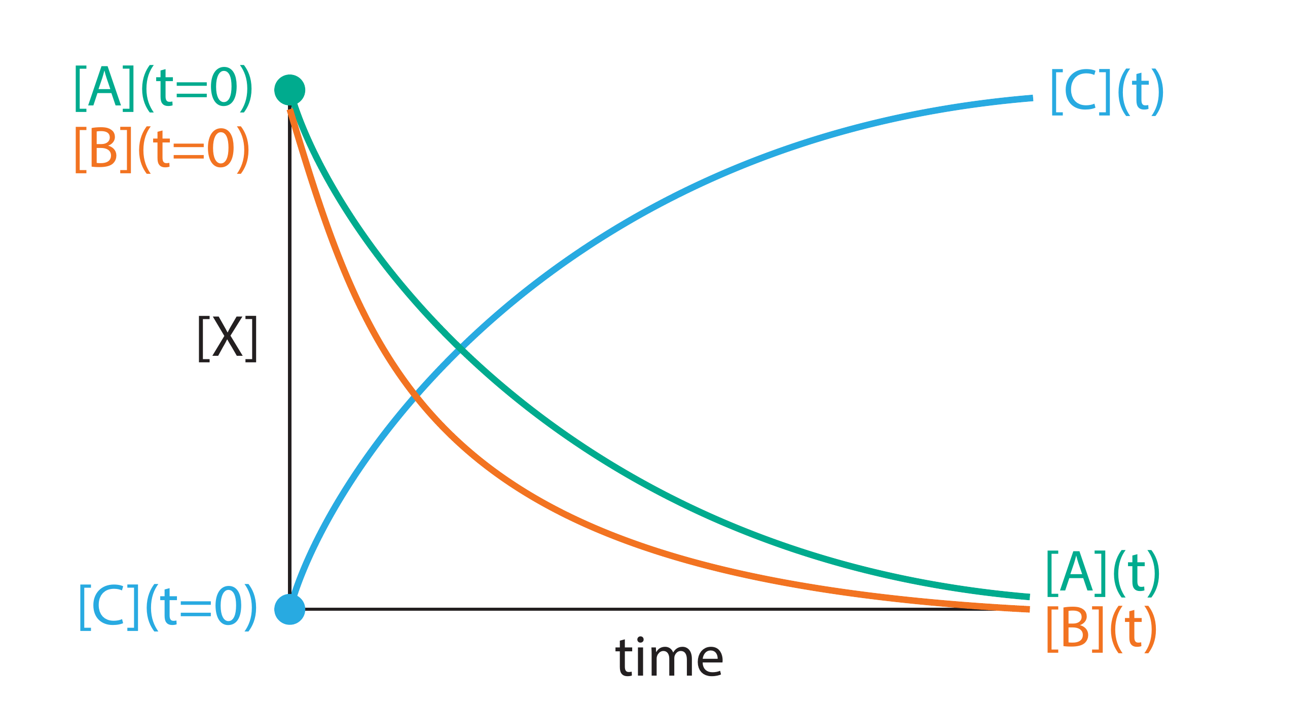
Figure 1.3: Concentration profiles for the reaction A + 2B → C. Species B is consumed twice as fast as A, reflecting the 2:1 stoichiometric ratio. The rate of formation of C equals the rate of consumption of A.
B is consumed twice as rapidly as A (Figure 1.3). This means that \(-\mathrm{d}[\mathrm{A}]/\mathrm{d}t\) and \(-\mathrm{d}[\mathrm{B}]/\mathrm{d}t\) give different numerical values, so our choice of which species to monitor would seem to affect the “rate” we report. To define a single, unambiguous reaction rate, we divide the rate of change of each species by its stoichiometric coefficient in the balanced equation. For A + 2B → C, this gives:
\[\text{rate} = -\frac{\mathrm{d}[\mathrm{A}]}{\mathrm{d}t} = -\frac{1}{2}\frac{\mathrm{d}[\mathrm{B}]}{\mathrm{d}t} = +\frac{\mathrm{d}[\mathrm{C}]}{\mathrm{d}t}\]
1.4 Mass Balance
But where do these stoichiometric factors come from? The answer follows from a simple principle: chemical reactions cannot create or destroy atoms, only rearrange them. This conservation of mass links the rates at which different species are produced and consumed.
Consider our simple reaction A → B. If each molecule of A converts into exactly one molecule of B, then at any time \(t\) the total number of molecules, and hence the total concentration, remains constant:
\[[\mathrm{A}]_t + [\mathrm{B}]_t = [\mathrm{A}]_0 + [\mathrm{B}]_0\]
If we start with pure A, so that \([\mathrm{B}]_0 = 0\), this simplifies to:
\[[\mathrm{A}]_t + [\mathrm{B}]_t = [\mathrm{A}]_0\]
Taking the derivative of both sides with respect to time:
\[\frac{\mathrm{d}[\mathrm{A}]}{\mathrm{d}t} + \frac{\mathrm{d}[\mathrm{B}]}{\mathrm{d}t} = 0\]
since the initial concentration \([\mathrm{A}]_0\) is a constant. Rearranging:
\[\frac{\mathrm{d}[\mathrm{B}]}{\mathrm{d}t} = -\frac{\mathrm{d}[\mathrm{A}]}{\mathrm{d}t}\]
This tells us that for this simple reaction, the rate of formation of B exactly equals the rate of consumption of A.
Now consider a reaction where one molecule of A produces two molecules of B:
\[\mathrm{A} \rightarrow 2\mathrm{B}\]
Here, conservation of mass does not imply conservation of moles—we gain one mole of molecules for every mole of A that reacts. To write a mass balance, we note that each A molecule that reacts produces two B molecules. If we define our “conserved quantity” in terms of B-equivalents, then one A is worth two B, giving:
\[2[\mathrm{A}]_t + [\mathrm{B}]_t = 2[\mathrm{A}]_0\]
Taking the derivative:
\[2\frac{\mathrm{d}[\mathrm{A}]}{\mathrm{d}t} + \frac{\mathrm{d}[\mathrm{B}]}{\mathrm{d}t} = 0\]
Rearranging:
\[\frac{\mathrm{d}[\mathrm{B}]}{\mathrm{d}t} = -2\frac{\mathrm{d}[\mathrm{A}]}{\mathrm{d}t}\]
This confirms that B is produced twice as fast as A is consumed—exactly what we expect from the stoichiometry. Denoting the reaction rate by \(\nu\), we can define a single rate that is independent of which species we monitor:
\[\nu = -\frac{\mathrm{d}[\mathrm{A}]}{\mathrm{d}t} = +\frac{1}{2}\frac{\mathrm{d}[\mathrm{B}]}{\mathrm{d}t}\]
For any reaction, mass balance leads to the general expression:
\[\nu = \frac{1}{\nu_\mathrm{X}}\frac{\mathrm{d}[\mathrm{X}]}{\mathrm{d}t}\]
where \(\nu_\mathrm{X}\) is the stoichiometric coefficient of species X, negative for reactants and positive for products. This relationship ensures that the reaction rate \(\nu\) has the same numerical value regardless of which species we use to measure it.
You should be able to: Given a balanced equation, write the reaction rate \(\nu\) in terms of the rate of change of concentration of any species, including the correct stoichiometric factors.
1.5 Rate Laws
Why do most reactions slow down as they progress? As reactant is consumed, fewer reactant molecules remain. With less reactant available, the rate of conversion into products falls. This suggests a general principle: the rate of a reaction depends on the concentrations of the reactants. The mathematical expression that captures this dependence is called a rate law.
Many reactions follow a simple rate law where the rate is proportional to the concentration of each reactant raised to some power:
\[\begin{equation} \nu = k[\mathrm{A}]^a[\mathrm{B}]^b[\mathrm{C}]^c \ldots \tag{1.1} \end{equation}\]
This expression contains several important quantities. The proportionality factor \(k\) is called the rate constant: a large rate constant means a fast reaction, a small one a slow reaction. The rate constant depends on temperature but not on concentration.
The exponents \(a\), \(b\), \(c\), etc. are called the order of reaction with respect to reactants A, B, C, etc., and their sum \((a + b + c + \ldots)\) is the overall reaction order. Orders need not be integers; they can be zero, fractional, or even negative.
The orders in a rate law need not reflect the stoichiometry of the overall reaction equation. For example:
\[\mathrm{H}_2 + \mathrm{I}_2 \rightarrow 2\mathrm{HI} \qquad \nu = k[\mathrm{H}_2][\mathrm{I}_2]\]
Here the orders, both 1, happen to match the stoichiometric coefficients. But consider:
\[3\mathrm{ClO}^- \rightarrow \mathrm{ClO}_3^- + 2\mathrm{Cl}^- \qquad \nu = k[\mathrm{ClO}^-]^2\]
The stoichiometric coefficient of ClO\(^-\) is 3, but the reaction is second order in ClO\(^-\).
Not all reactions follow a simple rate law. Consider the formation of hydrogen bromide:
\[\mathrm{H}_2 + \mathrm{Br}_2 \rightarrow 2\mathrm{HBr}\]
This has exactly the same stoichiometry as the H2 + I2 reaction above, so we might expect the same simple rate law. The experimentally determined rate law, however, is:
\[\nu = \frac{k[\mathrm{H}_2][\mathrm{Br}_2]^{1/2}}{1 + k'[\mathrm{HBr}]/[\mathrm{Br}_2]}\]
This is an example of a complex rate law: it cannot be written in the simple power-law form of Eqn. (1.1). The rate is proportional to \([\mathrm{H}_2]\), so the reaction is first order in H2, but the dependence on Br2 and HBr cannot be expressed as a simple power, and we cannot assign a single order with respect to either. Because the order is not defined for every species, the overall reaction order is also undefined.
1.6 Elementary Processes
What determines the form of a rate law? To answer this, we need to look at what happens at the molecular level.
When cyclopropane rearranges to propene, only a single molecule is involved: bonds within the ring break and reform to produce an open-chain isomer. When a hydrogen molecule collides with an iodine molecule and they react to form two molecules of HI, that collision is one event involving two molecules. Each of these is an elementary process (or elementary reaction): a single molecular event that cannot be broken down into simpler steps. Any chemical reaction, no matter how complex its overall stoichiometry, can be decomposed into a sequence of such steps.
We classify elementary processes by their molecularity, the number of reactant molecules that participate. A unimolecular process involves just one molecule, as in the cyclopropane isomerisation. A bimolecular process requires two molecules to collide and react, as in the formation of HI. Termolecular processes, where three molecules come together simultaneously, are rare because the probability of a simultaneous three-body collision is very low. These three cases are illustrated in Figure 1.4.
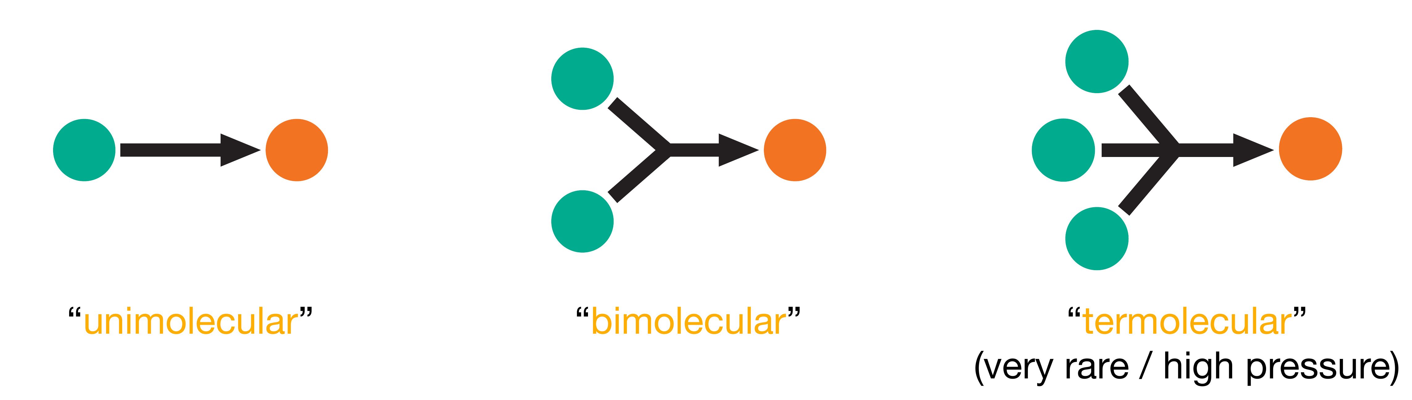
Figure 1.4: Schematic representation of elementary processes classified by molecularity. Unimolecular processes involve a single molecule (e.g., isomerisation or decomposition). Bimolecular processes involve collision between two molecules. Termolecular processes, involving simultaneous three-body collisions, are rare.
For elementary processes, and only for elementary processes, the rate law directly reflects the molecularity:
| Molecularity | Example | Rate Law |
|---|---|---|
| Unimolecular | \(\mathrm{A} \rightarrow \mathrm{P}\) | \(\nu = k[\mathrm{A}]\) |
| Bimolecular | \(\mathrm{A} + \mathrm{B} \rightarrow \mathrm{P}\) | \(\nu = k[\mathrm{A}][\mathrm{B}]\) |
| Bimolecular | \(2\mathrm{A} \rightarrow \mathrm{P}\) | \(\nu = k[\mathrm{A}]^2\) |
| Termolecular | \(\mathrm{A} + \mathrm{B} + \mathrm{C} \rightarrow \mathrm{P}\) | \(\nu = k[\mathrm{A}][\mathrm{B}][\mathrm{C}]\) |
This direct correspondence between molecularity and reaction order holds because an elementary process represents an actual molecular event. For a unimolecular process, the rate depends only on how many A molecules are present. For a bimolecular process, the rate depends on how often A and B molecules collide. Doubling the concentration of A doubles the number of A molecules available to collide; independently, doubling the concentration of B doubles the number of collision partners. The collision rate is therefore proportional to both \([\mathrm{A}]\) and \([\mathrm{B}]\).
1.7 Complex Reactions
Most reactions we encounter are not elementary processes but rather sequences of elementary steps. The H2 + Br2 reaction, for example, proceeds through a mechanism involving five elementary steps:
- \(\mathrm{Br}_2 \rightarrow 2\mathrm{Br}\)
- \(\mathrm{Br} + \mathrm{H}_2 \rightarrow \mathrm{H} + \mathrm{HBr}\)
- \(\mathrm{H} + \mathrm{Br}_2 \rightarrow \mathrm{Br} + \mathrm{HBr}\)
- \(\mathrm{H} + \mathrm{HBr} \rightarrow \mathrm{Br} + \mathrm{H}_2\)
- \(\mathrm{Br} + \mathrm{Br} \rightarrow \mathrm{Br}_2\)
Each elementary step follows a simple rate law determined by its molecularity, but the overall rate law for a complex reaction emerges from how these steps combine, which is why the overall rate law can be complicated. Conversely, when we observe a complex rate law, this tells us the reaction must proceed through multiple elementary steps.
For complex reactions, we cannot deduce the rate law from the stoichiometry alone; it must be determined experimentally. However, different mechanisms—different sequences of elementary steps—predict different overall rate laws. This gives us a powerful strategy: propose a mechanism, derive the rate law it predicts, and compare the prediction with experiment. Agreement supports the proposed mechanism; disagreement rules it out. Rate laws, therefore, are not merely descriptions of how fast a reaction proceeds—they provide a window into what is happening at the molecular level.
1.8 Units of the Rate Constant
The units of a rate constant depend on the overall order of the reaction. Since both sides of a rate equation must have the same dimensions, we can deduce the units of \(k\) from dimensional analysis. For a first-order reaction (\(\nu = k[\mathrm{A}]\)):
\[\underbrace{\mathrm{mol\,dm}^{-3}\mathrm{\,s}^{-1}}_{\text{rate}} = [k] \times \underbrace{\mathrm{mol\,dm}^{-3}}_{[\mathrm{A}]}\]
so \([k] = \mathrm{s}^{-1}\). Repeating this analysis for other orders gives:
| Overall order | Units of \(k\) |
|---|---|
| 0 | \(\mathrm{mol\,dm}^{-3}\,\mathrm{s}^{-1}\) |
| 1 | \(\mathrm{s}^{-1}\) |
| 2 | \(\mathrm{mol}^{-1}\,\mathrm{dm}^{3}\,\mathrm{s}^{-1}\) |
| 3 | \(\mathrm{mol}^{-2}\,\mathrm{dm}^{6}\,\mathrm{s}^{-1}\) |
The general pattern for overall order \(n\) is:
\[[k] = \mathrm{mol}^{1-n}\,\mathrm{dm}^{3(n-1)}\,\mathrm{s}^{-1}\]
Comparing rate constants only makes sense when they refer to the same order of reaction. A rate constant of \(10^6\,\mathrm{s}^{-1}\) for a first-order reaction cannot be directly compared with a rate constant of \(10^6\,\mathrm{mol}^{-1}\,\mathrm{dm}^{3}\,\mathrm{s}^{-1}\) for a second-order reaction.
You should be able to: Write the rate law for an elementary process given its molecularity, and determine the units of a rate constant given the overall reaction order.
We now have two mathematical descriptions of a reaction rate. The first defines rate as the derivative of a concentration: \(\nu = -\mathrm{d}[\mathrm{A}]/\mathrm{d}t\). The second expresses rate as a function of concentrations through the rate law: \(\nu = k[\mathrm{A}]^a[\mathrm{B}]^b\ldots\). Setting these equal gives a differential equation whose solution is the concentration profile, \([\mathrm{A}]_t\). Much of chemical kinetics involves moving between these two descriptions: from experimental concentration data to rate laws, and from rate laws to predicted concentration profiles. Because different mechanisms predict different rate laws, this interplay between measurement and prediction also provides a route from macroscopic observations to molecular-level understanding.
1.9 Key Concepts
- Thermodynamics tells us whether a reaction can occur; kinetics tells us how fast it proceeds.
- The reaction rate \(\nu\) is defined as the rate of change of concentration, with stoichiometric factors ensuring a single unambiguous value regardless of which species we monitor.
- Mass balance (conservation of mass) provides the physical basis for the stoichiometric factors in rate expressions.
- A rate law describes how the rate depends on concentrations. The reaction orders need not match the stoichiometric coefficients.
- Elementary processes are single molecular events (unimolecular, bimolecular, or termolecular). Only for elementary processes do the orders directly reflect the molecularity.
- Complex reactions consist of sequences of elementary steps. Their rate laws must be determined experimentally.
- Different mechanisms predict different rate laws. Comparing predicted and experimental rate laws provides insight into the molecular-level mechanism of a reaction.
- The units of a rate constant depend on the overall reaction order: for an \(n\)th-order reaction, \([k] = \mathrm{mol}^{1-n}\,\mathrm{dm}^{3(n-1)}\,\mathrm{s}^{-1}\).