Lecture 5 The Steady-State Approximation

For the mechanism A + B $\rightleftharpoons$ C $\rightarrow$ D, we can write down the differential rate equations for every species, but we cannot solve them analytically. The pre-equilibrium approximation gave us a tractable rate law for the special case $k_{-1} \gg k_2$, but what about other cases? And what about mechanisms with four, five, or six elementary steps? The bookkeeping needed to write down the rate equations grows, but the fundamental problem remains the same: the equations are coupled (the rate of change of one species depends on the concentrations of others) and there is no general analytical solution.

To make progress, we need approximation methods that work across a broad range of mechanisms. The steady-state approximation (SSA) is the most widely used such method in chemical kinetics. It applies whenever a reactive intermediate is consumed much faster than it is formed, and it reduces coupled differential equations to simple algebra.

5.1 The Idea Behind the Steady-State Approximation

In the consecutive reaction A $\rightarrow$ B $\rightarrow$ C from Lecture 4, the species B is formed in the first step and consumed in the second. It does not appear in the overall balanced equation (A $\rightarrow$ C), and when $k_2 \gg k_1$ it never accumulates to a significant concentration. B is an example of a reactive intermediate: a species that is produced and consumed during a reaction but is not present in the overall stoichiometry.

In many mechanisms, reactive intermediates like B are highly unstable — they are consumed almost as fast as they are produced, so their concentration remains small throughout the reaction.

If a reactive intermediate is consumed much faster than it is formed, two things follow. First, its concentration must remain small compared to those of the reactants and products; if it were to accumulate, the fast consumption step would rapidly remove the excess.

Second, after a brief initial period during which the intermediate builds up from zero, its concentration reaches a nearly constant value (a steady state) because any small increase in concentration is immediately counteracted by the fast consumption step.

The steady-state approximation exploits this. For a reactive intermediate I whose concentration is approximately constant, $\mathrm{d}[\mathrm{I}]/\mathrm{d}t \approx 0$. Under the SSA, we therefore set $\mathrm{d}[\mathrm{I}]/\mathrm{d}t = 0$:

\[\frac{\mathrm{d}[\mathrm{I}]}{\mathrm{d}t} = 0\]

This does not mean that $[\mathrm{I}] = 0$. The intermediate is present (it must be, because the reaction proceeds through it) but its concentration changes so slowly compared to the other species that we treat $\mathrm{d}[\mathrm{I}]/\mathrm{d}t$ as zero.

This step replaces a differential equation (which, together with the equations for the other species, forms a coupled system with no analytical solution) with an algebraic equation that we can solve by hand.

Figure 5.1 illustrates this for the consecutive reaction A $\rightarrow$ B $\rightarrow$ C when $k_1 \ll k_2$. Because B is consumed much faster than it is formed, it never accumulates to a significant concentration. After a brief initial rise, $[\mathrm{B}]$ remains low and nearly constant — precisely the conditions under which the SSA is valid.

$Concentration profiles for the consecutive reaction A → B → C when $k_1 \ll k_2$. The intermediate B rises briefly to a low concentration and then remains nearly constant as A is consumed. Because B is consumed (by the fast second step) much faster than it is formed (by the slow first step), it never accumulates to a significant concentration.$

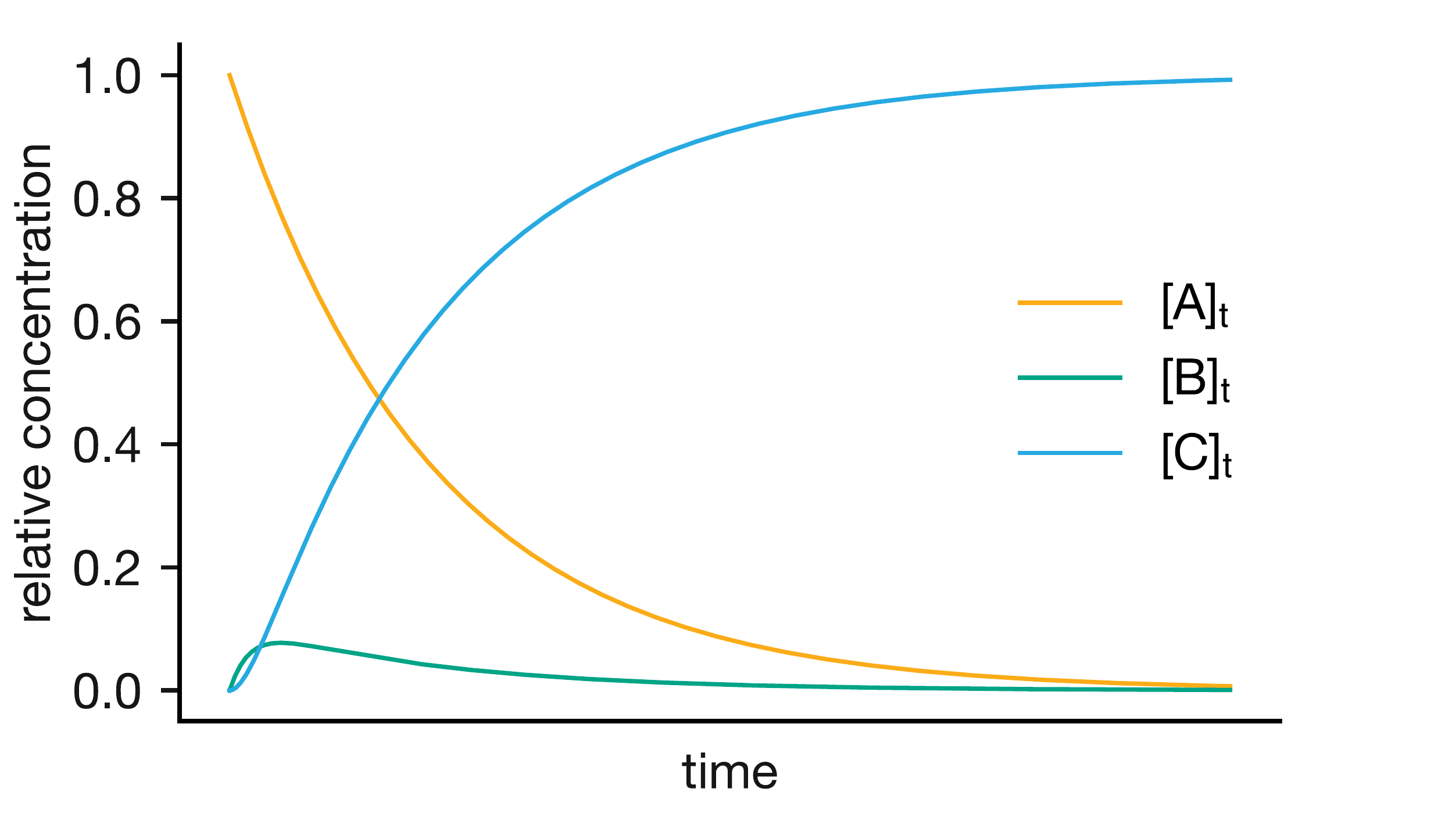
Figure 5.1: Concentration profiles for the consecutive reaction A → B → C when $k_1 \ll k_2$. The intermediate B rises briefly to a low concentration and then remains nearly constant as A is consumed. Because B is consumed (by the fast second step) much faster than it is formed (by the slow first step), it never accumulates to a significant concentration.

5.2 Applying the SSA: A + B ⇌ C → D

The pre-equilibrium approximation in Lecture 4 handled the mechanism below by assuming $k_{-1} \gg k_2$. The SSA makes no such assumption about which step is fast — it requires only that C is a short-lived intermediate. Consider again the mechanism

\[\mathrm{A} + \mathrm{B} \underset{k_{-1}}{\stackrel{k_1}{\rightleftharpoons}} \mathrm{C} \xrightarrow{k_2} \mathrm{D}\]

We want the overall rate of product formation, $\nu = \mathrm{d}[\mathrm{D}]/\mathrm{d}t = k_2[\mathrm{C}]$. But C is a short-lived reactive intermediate whose concentration we cannot measure directly. To compare this rate law with experimental data, we need to eliminate $[\mathrm{C}]$ and express $\nu$ in terms of species whose concentrations we can measure.

The rate equations for each species are:

\[\begin{align*} \frac{\mathrm{d}[\mathrm{A}]}{\mathrm{d}t} = \frac{\mathrm{d}[\mathrm{B}]}{\mathrm{d}t} &= -k_1[\mathrm{A}][\mathrm{B}] + k_{-1}[\mathrm{C}] \\ \frac{\mathrm{d}[\mathrm{C}]}{\mathrm{d}t} &= k_1[\mathrm{A}][\mathrm{B}] - k_{-1}[\mathrm{C}] - k_2[\mathrm{C}] \\ \frac{\mathrm{d}[\mathrm{D}]}{\mathrm{d}t} &= k_2[\mathrm{C}] \end{align*}\]

These are coupled differential equations: the equation for $[\mathrm{C}]$ depends on $[\mathrm{A}]$ and $[\mathrm{B}]$, and the equations for $[\mathrm{A}]$ and $[\mathrm{B}]$ depend on $[\mathrm{C}]$. We can write down the rate equations for any mechanism, but coupled systems like this have no simple analytical solution.

If C is a short-lived, reactive intermediate, however, we can apply the SSA. Setting $\mathrm{d}[\mathrm{C}]/\mathrm{d}t = 0$ gives:

\[k_1[\mathrm{A}][\mathrm{B}] - k_{-1}[\mathrm{C}] - k_2[\mathrm{C}] = 0\]

This is now an algebraic equation: the coupled differential equation for $[\mathrm{C}]$ has been replaced by an expression we can rearrange directly. Solving for the steady-state concentration of C:

\[k_1[\mathrm{A}][\mathrm{B}] = (k_{-1} + k_2)[\mathrm{C}]\]

\[[\mathrm{C}]_\mathrm{ss} = \frac{k_1[\mathrm{A}][\mathrm{B}]}{k_{-1} + k_2}\]

The overall rate of product formation is then:

\[\begin{equation} \nu = \frac{\mathrm{d}[\mathrm{D}]}{\mathrm{d}t} = k_2[\mathrm{C}]_\mathrm{ss} = \frac{k_1 k_2[\mathrm{A}][\mathrm{B}]}{k_{-1} + k_2} \tag{5.1} \end{equation}\]

This is the SSA rate law for this mechanism. It is second order overall (first order in A, first order in B), with an effective rate constant $k_\mathrm{obs} = k_1 k_2/(k_{-1} + k_2)$. This is an approximate result, relying on the assumption that C reaches a steady state, but it gives us a closed-form rate law expressed entirely in terms of species whose concentrations we can measure.

5.2.1 Pre-Equilibrium and Irreversible Limits

The denominator $(k_{-1} + k_2)$ in Eqn. (5.1) has a direct physical meaning: it represents the two competing fates of the intermediate C. Once formed, C can either revert to A + B (with rate constant $k_{-1}$) or proceed to D (with rate constant $k_2$). The SSA is valid whenever the combined rate of these consumption processes is much faster than the rate of formation, so that C is consumed almost as soon as it appears and never accumulates to a significant concentration.

The two limiting cases correspond to which fate dominates.

If reversion to reactants is the dominant fate ($k_{-1} \gg k_2$), the denominator is dominated by $k_{-1}$:

\[(k_{-1} + k_2) \approx k_{-1}\]

The rate law (Eqn. (5.1)) then simplifies to:

\[\nu \approx \frac{k_1 k_2}{k_{-1}}[\mathrm{A}][\mathrm{B}]\]

This is exactly the pre-equilibrium rate law from Lecture 4 (Eqn. (4.4)). Physically, C reverts to A + B many times before occasionally proceeding to D. The first step has time to reach equilibrium, and the slow second step controls the overall rate. The effective rate constant $k_\mathrm{obs} = k_1 k_2/k_{-1}$ depends on all three elementary rate constants.

If instead the forward reaction to product dominates ($k_2 \gg k_{-1}$), the denominator is dominated by $k_2$:

\[(k_{-1} + k_2) \approx k_2\]

The $k_2$ terms cancel, and the rate law reduces to:

\[\nu \approx k_1[\mathrm{A}][\mathrm{B}]\]

Now the overall rate depends only on $k_1$. Once C is formed, it proceeds to D so rapidly that reversion to A + B is negligible. The first step is made irreversible by the fast second step, even though it is intrinsically reversible. The first step is therefore rate-determining, and the rate law is simply the rate of the first elementary step.

The two limits give the same functional form (both are second order in A and B) but different effective rate constants: $k_1 k_2/k_{-1}$ in the pre-equilibrium limit and $k_1$ in the irreversible limit.

We can test how well the SSA predicts the product concentration by comparing the approximate $[\mathrm{D}]$ (from the SSA rate law) with the exact numerical solution (Figure 5.2).

Exact concentration profiles for the mechanism A + B ⇌ C → D (solid lines), together with the prediction for [D] from the SSA rate law (dashed line). The intermediate C remains at low concentration throughout, consistent with the steady-state assumption. The SSA prediction closely matches the exact solution, with only a small discrepancy at short times while [C] builds up to its steady-state value.

Figure 5.2: Exact concentration profiles for the mechanism A + B ⇌ C → D (solid lines), together with the prediction for [D] from the SSA rate law (dashed line). The intermediate C remains at low concentration throughout, consistent with the steady-state assumption. The SSA prediction closely matches the exact solution, with only a small discrepancy at short times while [C] builds up to its steady-state value.

The agreement between the SSA prediction and the exact solution is much closer than for the pre-equilibrium comparison in Lecture 4 (Figure 4.5). Under SSA conditions, the intermediate $[\mathrm{C}]$ remains small throughout the reaction, so it reaches its steady-state concentration almost immediately and the induction period is negligibly short.

Where the SSA does break down is at the very start of the reaction. The logic is straightforward: we derived the rate law by assuming that $[\mathrm{C}]$ does not change, so the approximation is worst wherever $[\mathrm{C}]$ changes most, and that is during the initial transient as the intermediate builds up from zero to its steady-state value. Once the steady state is established, the approximation becomes increasingly accurate.

You should be able to: Apply the steady-state approximation to the mechanism A + B ⇌ C → D by setting $\mathrm{d}[\mathrm{C}]/\mathrm{d}t = 0$, derive the rate law $\nu = k_1 k_2[\mathrm{A}][\mathrm{B}]/(k_{-1} + k_2)$, and show that the pre-equilibrium result is recovered when $k_{-1} \gg k_2$.

5.3 A Second Example: A ⇌ B, B + C → D

A second example shows how the SSA can produce rate laws with richer concentration dependence. Consider the mechanism

\[\mathrm{A} \underset{k_{-1}}{\stackrel{k_1}{\rightleftharpoons}} \mathrm{B} \qquad \mathrm{B} + \mathrm{C} \xrightarrow{k_2} \mathrm{D}\]

Here, A isomerises reversibly to form a reactive intermediate B, which then reacts with a second species C to give the product D. The overall rate of product formation is $\nu = k_2[\mathrm{B}][\mathrm{C}]$, but B is a short-lived reactive intermediate whose concentration we cannot measure directly. As before, we need to eliminate $[\mathrm{B}]$ and express $\nu$ in terms of measurable concentrations.

The rate equation for B is:

\[\frac{\mathrm{d}[\mathrm{B}]}{\mathrm{d}t} = k_1[\mathrm{A}] - k_{-1}[\mathrm{B}] - k_2[\mathrm{B}][\mathrm{C}]\]

Setting $\mathrm{d}[\mathrm{B}]/\mathrm{d}t = 0$ and solving for $[\mathrm{B}]_\mathrm{ss}$:

\[k_1[\mathrm{A}] = [\mathrm{B}](k_{-1} + k_2[\mathrm{C}])\]

\[[\mathrm{B}]_\mathrm{ss} = \frac{k_1[\mathrm{A}]}{k_{-1} + k_2[\mathrm{C}]}\]

The overall rate of product formation is then:

\[\begin{equation} \nu = k_2[\mathrm{B}]_\mathrm{ss}[\mathrm{C}] = \frac{k_1 k_2[\mathrm{A}][\mathrm{C}]}{k_{-1} + k_2[\mathrm{C}]} \tag{5.2} \end{equation}\]

In this rate law, $[\mathrm{C}]$ appears in both the numerator and the denominator. As a result, the rate is not simply proportional to $[\mathrm{C}]$ — there is no well-defined order with respect to C. (The rate is, however, always first order in A.) This is a good example of a mechanism that gives rise to a rate law that cannot be expressed as a simple power law $\nu = k[\mathrm{A}]^m[\mathrm{C}]^n$.

5.3.1 Concentration-Dependent Limiting Behaviour

As before, the denominator represents two competing fates for the intermediate. But here there is an important difference: one of the terms, $k_2[\mathrm{C}]$, depends on the concentration of C, not just on rate constants.

If reversion to A dominates ($k_{-1} \gg k_2[\mathrm{C}]$), the denominator is dominated by $k_{-1}$:

\[(k_{-1} + k_2[\mathrm{C}]) \approx k_{-1}\]

The rate law (Eqn. (5.2)) then simplifies to:

\[\nu \approx \frac{k_1 k_2}{k_{-1}}[\mathrm{A}][\mathrm{C}]\]

The reaction is first order in A, first order in C, and second order overall. Physically, B reverts to A many times before it encounters a molecule of C. The first step is at equilibrium, and the second step is rate-determining. The effective rate constant is $k_\mathrm{obs} = k_1 k_2/k_{-1} = Kk_2$, where $K = k_1/k_{-1}$ is the equilibrium constant for the first step.

If instead the reaction with C dominates ($k_2[\mathrm{C}] \gg k_{-1}$), the denominator is dominated by $k_2[\mathrm{C}]$:

\[(k_{-1} + k_2[\mathrm{C}]) \approx k_2[\mathrm{C}]\]

The $k_2[\mathrm{C}]$ terms cancel, and the rate law reduces to:

\[\nu \approx k_1[\mathrm{A}]\]

The reaction is first order in A and zero order in C — the rate does not depend on $[\mathrm{C}]$ at all. This limit is reached whenever $k_2[\mathrm{C}] \gg k_{-1}$, either because the concentration of C is large or because $k_2$ itself is large. In either case, every molecule of B that forms reacts with C almost immediately, and the bottleneck is the rate at which B is produced from A.

Because the comparison involves the product $k_2[\mathrm{C}]$ rather than just a rate constant, it is possible to switch between these two regimes experimentally by varying $[\mathrm{C}]$. At low $[\mathrm{C}]$, where $k_{-1} \gg k_2[\mathrm{C}]$, the reaction is first order in C and second order overall. At high $[\mathrm{C}]$, where $k_2[\mathrm{C}] \gg k_{-1}$, the reaction becomes zero order in C and first order overall.

This is a concrete, testable prediction: the SSA tells us not just what the rate law is, but how the apparent order should change with experimental conditions. If a proposed mechanism follows this pattern, we can test it by measuring the rate at different concentrations of C and checking whether the order shifts as predicted.

You should be able to: Apply the SSA to a mechanism with a reactive intermediate (such as A ⇌ B, B + C → D), derive the resulting rate law, and identify the limiting cases by examining which terms dominate in the denominator.

5.4 SSA versus Pre-Equilibrium

Both the pre-equilibrium approximation and the steady-state approximation handle reactive intermediates, but they make different assumptions and apply in different regimes. The pre-equilibrium approximation assumes that the first step genuinely reaches equilibrium before the slow step proceeds, requiring $k_{-1} \gg k_2$. It gives a simple derivation and a clear physical picture, but applies only in this specific limit. The SSA assumes only that the intermediate’s concentration reaches a quasi-steady value, which can happen whether or not the first step is at equilibrium. It therefore covers a broader range of conditions and reduces to the pre-equilibrium result when $k_{-1} \gg k_2$.

In practice: if we are told (or can justify) that the first step is a fast equilibrium, the pre-equilibrium approach is quicker and gives the same answer. If no such information is given, or if we need a result that covers different limiting cases, the SSA is the better choice.

The consecutive reaction A $\to$ B $\to$ C from Lecture 4, in the case $k_2 \gg k_1$ where B is a short-lived intermediate, provides a useful check. The rate equation for B is:

\[\frac{\mathrm{d}[\mathrm{B}]}{\mathrm{d}t} = k_1[\mathrm{A}] - k_2[\mathrm{B}]\]

Setting this to zero gives $k_1[\mathrm{A}] = k_2[\mathrm{B}]_\mathrm{ss}$, so $[\mathrm{B}]_\mathrm{ss} = k_1[\mathrm{A}]/k_2$. The overall rate of product formation is then:

\[\nu = k_2[\mathrm{B}]_\mathrm{ss} = k_2 \times \frac{k_1[\mathrm{A}]}{k_2} = k_1[\mathrm{A}]\]

This is first order with rate constant $k_1$, exactly the rate-limiting step result from Lecture 4. The SSA provides a more direct route to the same conclusion.

5.5 Key Concepts

The steady-state approximation (SSA) sets $\mathrm{d}[\mathrm{I}]/\mathrm{d}t = 0$ for a reactive intermediate I. This does not mean $[\mathrm{I}] = 0$; it means $[\mathrm{I}]$ is approximately constant after a brief initial transient.
The SSA is valid when a reactive intermediate is consumed much faster than it is formed, so that its concentration remains small and approximately constant throughout the reaction.
Applying the SSA converts coupled differential equations (which generally have no analytical solution) into algebraic equations, allowing us to eliminate unmeasurable reactive intermediates from the rate law.
For the mechanism A + B ⇌ C → D, the SSA gives $\nu = k_1 k_2[\mathrm{A}][\mathrm{B}]/(k_{-1} + k_2)$, which contains both the pre-equilibrium limit ($k_{-1} \gg k_2$) and the irreversible limit ($k_2 \gg k_{-1}$) as special cases.
Some mechanisms produce rate laws where a species appears in both the numerator and denominator, giving no well-defined reaction order. The SSA naturally captures this behaviour.
The SSA is more general than the pre-equilibrium approximation and reduces to it as a special case. Use the SSA when you know (or can argue) that an intermediate is short-lived, but cannot justify a specific relationship between the rate constants.