Lecture 1 Introduction to Monte Carlo Methods

1.1 Introduction to Averaging & Sampling

Chemistry is fundamentally a statistical science. Macroscopic properties such as pressure, temperature, and heat capacity emerge from the collective behaviour of approximately $10^{23}$ atoms or molecules. These observable quantities represent averages over an immense number of microscopic states. A central challenge in computational chemistry is how to accurately estimate these macroscopic properties without having to evaluate every possible molecular arrangement (Figure 1.1).

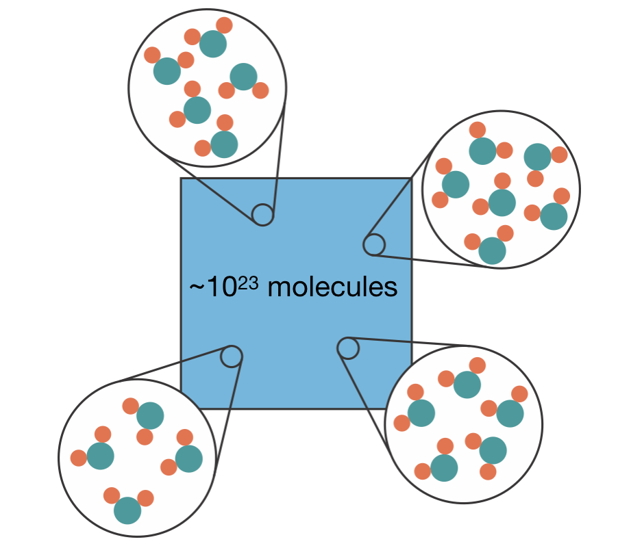
$A macroscopic chemical system contains approximately $10^{23}$ molecules. Zooming in at different points reveals different molecular arrangements — these are the microscopic configurations whose properties we need to average.$

Figure 1.1: A macroscopic chemical system contains approximately $10^{23}$ molecules. Zooming in at different points reveals different molecular arrangements — these are the microscopic configurations whose properties we need to average.

1.1.1 The Statistical Nature of Chemical Systems

When we measure properties of chemical systems in the laboratory, we observe the average behaviour of countless molecules over the duration of our measurement. Even the simplest systems—gases, liquids, or solids—involve enormous numbers of possible arrangements of atoms, with molecules constantly moving, rotating, and vibrating at finite temperatures. To predict these macroscopic measurements, we need to average our property of interest over all possible configurations, weighting each by the probability of it occurring:

\[\begin{equation} \langle A \rangle = \sum_{\mathbf{r}} A(\mathbf{r}) \times P(\mathbf{r}) \end{equation}\]

Here the angle brackets $\langle \cdot \rangle$ denote an average value, $\mathbf{r}$ represents a particular configuration of the system, and $P(\mathbf{r})$ is the probability of finding the system in that configuration.

1.1.2 Probability Distributions

$P(\mathbf{r})$ is a probability distribution—it specifies, for each possible value of some quantity, how likely that value is. Rolling a fair six-sided die, for example, gives each number (1–6) a probability of 1/6 (Figure 1.2). Because the possible values are countable, this is a discrete distribution. A distribution where every value is equally likely is called uniform.

Figure 1.2: A uniform discrete distribution: each face of a fair die has equal probability 1/6.

Not all discrete distributions are uniform: for example, flipping four (fair) coins gives probabilities of 1/16, 4/16, 6/16, 4/16, and 1/16 for 0, 1, 2, 3, and 4 heads respectively. The most probable outcome is 2 heads and 2 tails, because this result can happen the most ways (six) (Figure 1.3).

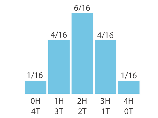
A non-uniform discrete distribution: the number of heads in four coin flips. The middle outcomes are more probable because there are more ways to arrange them.

Figure 1.3: A non-uniform discrete distribution: the number of heads in four coin flips. The middle outcomes are more probable because there are more ways to arrange them.

For any discrete distribution, the sum of probabilities across all possible outcomes must equal 1:

\[\sum_i P(i) = 1\]

Not all quantities have countable values. The Maxwell–Boltzmann speed distribution (Figure 1.4), for example, describes the probability of finding a molecule travelling at a particular speed—the speed can take any value in a continuous range. For these continuous distributions, the probability of a value falling in a specific range equals the area under the curve over that range.

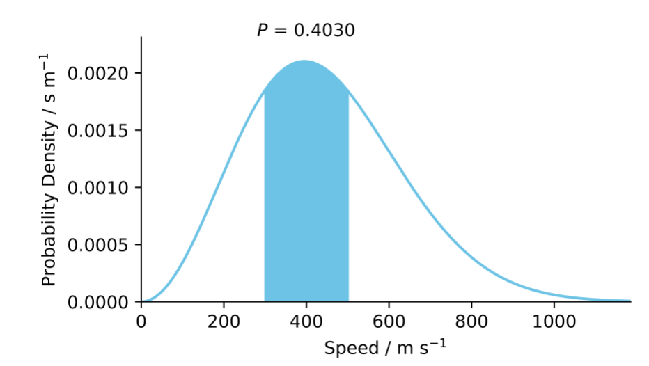
$The Maxwell--Boltzmann speed distribution, a continuous probability density function. The shaded area gives the probability of finding a molecule with speed between 300 and 500 m s$^{-1}$: the area under the curve in this range is approximately 0.40.$

Figure 1.4: The Maxwell–Boltzmann speed distribution, a continuous probability density function. The shaded area gives the probability of finding a molecule with speed between 300 and 500 m s$^{-1}$: the area under the curve in this range is approximately 0.40.

For continuous distributions, the integral over the entire domain must equal 1:

\[\int_{-\infty}^{\infty} P(x) \, \mathrm{d}x = 1\]

This normalisation requirement—that probabilities sum or integrate to 1—reflects the certainty that the system must exist in some state.

The average (expected value) of any property A is calculated by weighting each possible value by its probability. For discrete distributions:

\[\langle A \rangle = \sum_i A_i\, P_i\]

This is exactly the weighted sum we wrote down earlier for chemical systems. For continuous distributions, the equivalent expression is an integral:

\[\langle A \rangle = \int_{-\infty}^{\infty} A(x) \times P(x) \, \mathrm{d}x\]

1.1.3 The Boltzmann Distribution

In chemical systems, the probability distribution that governs molecular configurations is the Boltzmann distribution:

\[\begin{equation} P(\mathbf{r}) \propto \exp(-U(\mathbf{r})/k_\mathrm{B}T) \end{equation}\]

Here, $U(\mathbf{r})$ is the potential energy of configuration $\mathbf{r}$, $k_\mathrm{B}$ is Boltzmann’s constant, and $T$ is the temperature.

This relationship reveals a fundamental principle: lower-energy configurations are exponentially more probable than higher-energy ones (Figure 1.5). At room temperature (298 K), a configuration that is 6 kJ/mol higher in energy is approximately 10 times less probable than the minimum energy state, and contributes approximately 10 times less to any thermodynamic averages.¹ At high temperatures, higher-energy configurations become more accessible and the distribution flattens; at low temperatures, the lowest-energy states dominate increasingly strongly.

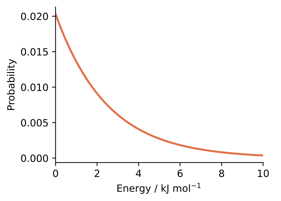
The Boltzmann distribution at room temperature (298 K). Lower-energy configurations have exponentially higher probability than higher-energy ones.

Figure 1.5: The Boltzmann distribution at room temperature (298 K). Lower-energy configurations have exponentially higher probability than higher-energy ones.

For $P(\mathbf{r})$ to be a valid probability distribution, the probabilities must sum to 1:

\[\begin{equation} \sum_i P(\mathbf{r}_i) = 1 \end{equation}\]

We achieve this by including a normalisation constant, $Z$:

\[\begin{equation} P(\mathbf{r}) = \frac{\exp(-U(\mathbf{r})/k_\mathrm{B}T)}{Z} \end{equation}\]

This constant $Z$ is called the “partition function”, defined as:

\[\begin{equation} Z = \sum_{\mathbf{r}} \exp(-U(\mathbf{r})/k_\mathrm{B}T) \end{equation}\]

1.1.4 The Computational Challenge

The mathematical framework presented above appears to provide everything we need to calculate any thermodynamic property of our system. In principle, we can generate all possible configurations, and for each one compute the property of interest, $A$, and the energy. From the calculated energies, we compute the partition function, and hence the probabilities, $P(\mathbf{r}_i)$, for each configuration. We then compute our thermodynamic property as a weighted sum over all configurations.

In practice, however, computing this sum over all possible states is impossible for any realistic chemical system. Figure 1.6 shows a simple example problem: a $10 \times 10$ array of surface sites with 50 adsorbed molecules. Even this “toy” problem has far too many configurations to compute each one individually: considering all possible arrangements of the adsorbed molecule gives $10^{29}$ possible configurations; this is more than the number of stars in the observable universe (Figure 1.7).

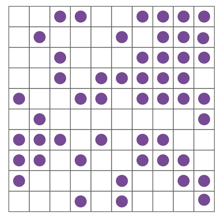
$A single configuration of 50 molecules adsorbed on a $10 \times 10$ lattice of surface sites.$

Figure 1.6: A single configuration of 50 molecules adsorbed on a $10 \times 10$ lattice of surface sites.

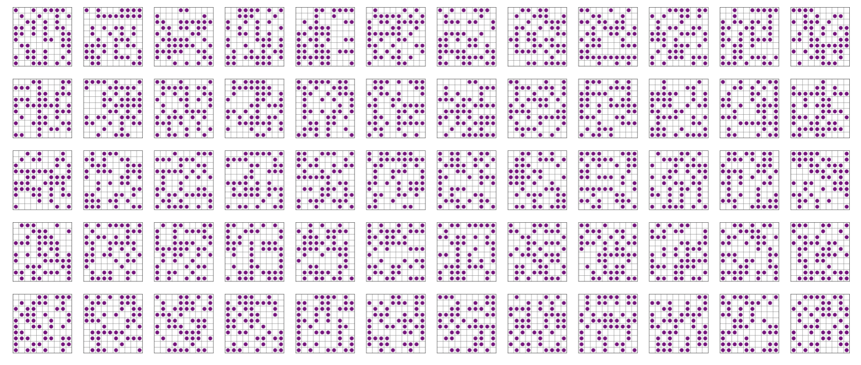
$A small selection of the approximately $10^{29}$ possible configurations of 50 molecules on a $10 \times 10$ lattice. Direct enumeration of all configurations is computationally intractable.$

Figure 1.7: A small selection of the approximately $10^{29}$ possible configurations of 50 molecules on a $10 \times 10$ lattice. Direct enumeration of all configurations is computationally intractable.

1.2 The Solution: Statistical Sampling

Instead, we can estimate the sum through sampling—selecting a representative subset of configurations (Figure 1.8), evaluating our property of interest for these samples, and calculating their average.

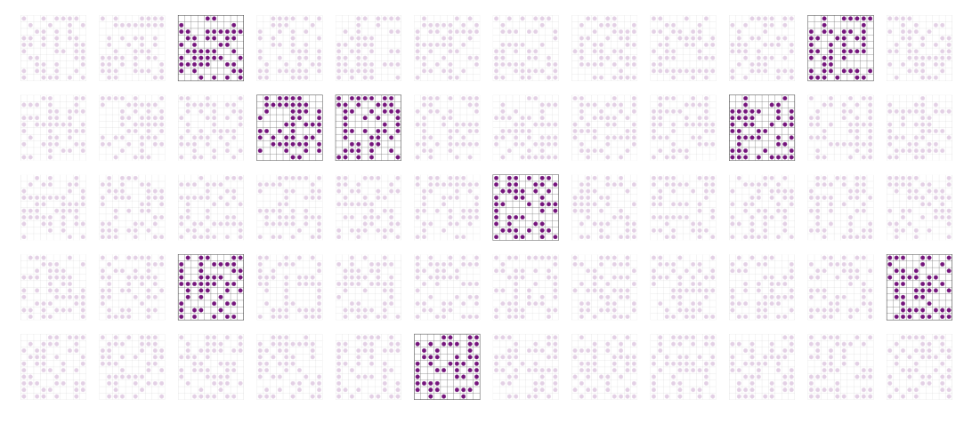
Rather than evaluating all possible configurations, we select a representative subset (highlighted) and use these to estimate the average.

Figure 1.8: Rather than evaluating all possible configurations, we select a representative subset (highlighted) and use these to estimate the average.

This concept of sampling is fundamental throughout science and statistics. Consider estimating the average height of people in the UK. Measuring everyone’s height is impractical, but we can measure a representative sample and use that sample’s average as an estimate of the true population average. The key requirement is that our sample must be representative—it should reflect the true probability distribution of the property we’re measuring. For instance, sampling players arriving for a basketball tournament would likely produce a significant overestimate of the average UK height, as basketball players tend to be taller than the general population. In contrast, measuring the heights of people passing by on a street corner on a Saturday afternoon would provide a more representative sample of the UK population.

When we sample directly from the correct probability distribution (for example, by randomly selecting UK citizens with equal probability), we can use simple averaging without additional weighting factors. However, if our sampling method is biased (like measuring only basketball players), we would need to apply appropriate weighting corrections.

This principle applies to chemical systems as well. If we could generate configurations directly according to the Boltzmann distribution, calculating thermodynamic properties would simply require averaging the property values:

\[\begin{equation} \langle A \rangle \approx \frac{1}{N} \sum_{i=1}^{N} A(\mathbf{r}_i) \end{equation}\]

where the configurations $\mathbf{r}_i$ are selected with probability proportional to $\exp(-U(\mathbf{r}_i)/k_\mathrm{B}T)$.

1.3 Two Approaches to Sampling

Computational chemistry has two principal approaches to this sampling problem:

1.3.1 Sampling using Molecular Dynamics

Molecular Dynamics (MD) simulates atomic motion by calculating the forces on every atom and numerically integrating Newton’s equations of motion. When performed in the canonical (NVT) ensemble, MD generates trajectories that naturally sample configurations according to their Boltzmann probabilities—like measuring people’s heights one by one as they file through a doorway. When a simulation trajectory visits a suitably representative set of configurations in the relevant regions of configuration space, the time average provides a good approximation of the desired ensemble average:

\[\begin{equation} \langle A \rangle \approx \frac{1}{M} \sum_{i=1}^{M} A(\mathbf{r}_i) \end{equation}\]

where $M$ is the number of time steps.

However, the effectiveness of MD sampling depends on the system’s energy landscape. Consider a protein folding example: if high energy barriers separate different conformational states, the protein may remain trapped in one conformation for the entire simulation duration. The resulting time average would reflect only a small subset of the relevant configuration space, not the true equilibrium ensemble.

Timescales present another challenge. Many important chemical processes occur on microsecond to second timescales, while individual MD time steps typically represent femtoseconds. This creates a fundamental gap between simulation capability and the time needed to observe certain phenomena. For instance, studying a slow conformational change or a rare reaction event may require prohibitively long simulation times.

Additionally, MD requires that forces can be calculated for every atom in the system. For problems with discrete variables—lattice models with discrete site occupancies, magnetic materials with fixed spin orientations—there are no continuous coordinates to differentiate and therefore no forces to integrate.

1.3.2 Sampling using Monte Carlo methods

Monte Carlo (MC) methods take a different approach: instead of following a physical trajectory, they use random numbers to select configurations directly—like picking people at random from a crowd rather than waiting for them to file past. Each configuration is selected, the property of interest is evaluated, and the results are averaged. Because the sampling does not depend on forces or equations of motion, MC methods apply equally well to continuous and discrete systems—lattice models, spin systems, or any problem where dynamical simulation would be awkward or impossible.

1.4 Monte Carlo with Uniform Sampling

Sampling configurations according to the Boltzmann distribution turns out to be the hard part of Monte Carlo simulation, and is the subject of the next two lectures. The underlying idea—using random samples to estimate the result of a calculation—is best seen first in simpler settings where each possible outcome has an equal probability of occurring.

1.4.1 Estimating π by Monte Carlo Integration

One of the simplest demonstrations of Monte Carlo methods is estimating the value of $\pi$. Consider a circle with radius 1 inscribed inside a square with side length 2 (Figure 1.9). The area of the circle is $\pi$, while the area of the square is 4. Therefore, the ratio of these areas is $\pi/4$.

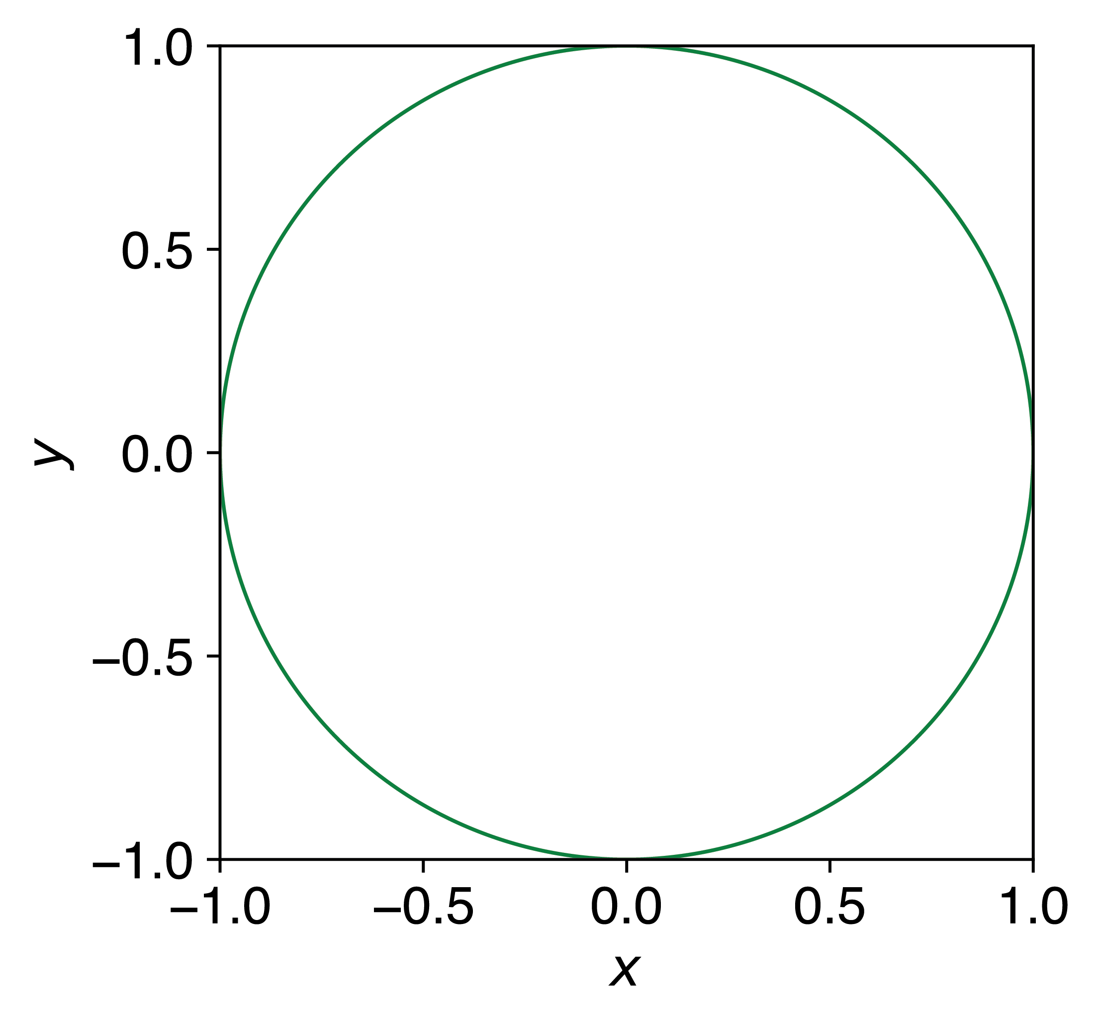
$A circle of radius 1 inscribed inside a square of side length 2. The ratio of the circle's area to the square's area is $\pi/4$.$

Figure 1.9: A circle of radius 1 inscribed inside a square of side length 2. The ratio of the circle’s area to the square’s area is $\pi/4$.

We can estimate this ratio by randomly placing points within the square and counting what fraction fall inside the circle. The procedure involves generating $N$ random points with coordinates $(x,y)$, where $x$ and $y$ are uniformly distributed between −1 and 1. We then count how many points $M$ satisfy $x^2 + y^2 \leq 1$, which indicates they fall within the circle. The estimate for $\pi$ is given by: $\pi \approx 4 \times M/N$. Figure 1.10 shows how the estimate converges as the number of samples increases.

$Estimating $\pi$ by Monte Carlo sampling. Random points are generated uniformly within a square of side length 2. Points falling inside the inscribed unit circle (red) and outside (blue) are counted, and $\pi$ is estimated from the ratio $4 \times M/N$. As the number of samples increases, the estimate converges towards the true value of $\pi$.$

Figure 1.10: Estimating $\pi$ by Monte Carlo sampling. Random points are generated uniformly within a square of side length 2. Points falling inside the inscribed unit circle (red) and outside (blue) are counted, and $\pi$ is estimated from the ratio $4 \times M/N$. As the number of samples increases, the estimate converges towards the true value of $\pi$.

This approach demonstrates how random sampling can solve a deterministic problem.

1.4.2 Monte Carlo Integration

A more practical application is numerical integration. Consider finding the average value of $\sin^2(x)$ over the interval $[0,\pi]$ (Figure 1.11).

Mathematically, this average is defined as:

\[\begin{equation} \text{Average value} = \frac{1}{\pi} \times \int_0^{\pi} \sin^2(x) dx \end{equation}\]

The analytical solution to this integral is 1/2.

$The function $\sin^2(x)$ over $[0, \pi]$ (solid curve), with the shaded area representing the integral. The dashed line shows the exact average value of 1/2.$

Figure 1.11: The function $\sin^2(x)$ over $[0, \pi]$ (solid curve), with the shaded area representing the integral. The dashed line shows the exact average value of 1/2.

We can estimate this average using Monte Carlo methods, by generating uniform random $x$-values between 0 and $\pi$, calculating $\sin^2(x)$ for each point, and then averaging these results. For example, suppose we generate five random values: $x = 0.50, 1.20, 2.10, 0.85, 2.70$. Evaluating $\sin^2(x)$ for each gives $0.230, 0.869, 0.745, 0.564, 0.183$, with an average of $0.518$—already close to the exact value of $0.500$ with just five samples.

This procedure can be generalised to estimate any definite integral:

\[\begin{equation} \int_a^b f(x)\,\mathrm{d}x \approx (b-a) \times \frac{1}{N} \sum_{i=1}^{N} f(x_i) \end{equation}\]

where $x_1$, $x_2$, …, $x_N$ are uniform random numbers between $a$ and $b$. The factor $(b-a)$ converts the average value of $f(x)$ into the area under the curve: the integral equals the average height of the function multiplied by the width of the interval.

The strength of this approach becomes apparent when dealing with multi-dimensional integrals, where traditional numerical methods become exponentially more expensive as dimensionality increases.

1.5 Statistical Uncertainty in Monte Carlo Methods

Unlike deterministic methods, which give the same answer every time, Monte Carlo methods produce slightly different results each time we run them with a different sequence of random numbers. We must therefore treat Monte Carlo results as estimates with associated uncertainty.

The precision of these estimates improves as we increase the number of samples. Statistical uncertainty decreases proportionally to $1/\sqrt{N}$, where $N$ is the number of random samples (Figure 1.12). To reduce the uncertainty by half, we need to use four times as many samples. This scaling behaviour is characteristic of random sampling methods and remains independent of the dimensionality of the problem—a significant advantage in high-dimensional applications.

$Convergence of Monte Carlo estimates of $\pi$. Each green trace represents an independent simulation. As the number of samples increases, all estimates converge towards the true value (dashed line), with the spread of estimates narrowing as $1/\sqrt{N}$.$

Figure 1.12: Convergence of Monte Carlo estimates of $\pi$. Each green trace represents an independent simulation. As the number of samples increases, all estimates converge towards the true value (dashed line), with the spread of estimates narrowing as $1/\sqrt{N}$.

When reporting Monte Carlo results, always include the associated uncertainties alongside the estimated values.

1.6 Summary

Monte Carlo methods use random sampling to estimate quantities that would be intractable to calculate exactly. Uniform random sampling can estimate $\pi$ (by counting points inside a circle) and evaluate definite integrals (by averaging function values at random points). These estimates carry statistical uncertainty that decreases as $1/\sqrt{N}$, so more samples give more precise results.

All of these examples used uniform sampling—each point was equally likely. For chemical systems, where configurations follow the Boltzmann distribution, we need a way to sample non-uniformly, without having to calculate the partition function $Z$.

Since the energy is expressed per mole, we use the gas constant $R = N_\mathrm{A} k_\mathrm{B} = 8.314$ J mol$^{-1}$ K$^{-1}$ in place of $k_\mathrm{B}$: $\exp(-6000/(8.314 \times 298)) \approx 1/10$.↩︎